Adiabatic Quantum Computing for Random Satisfiability Problemsappeared in Phys Rev A 67, 022314 (2003)
Abstract
The discrete formulation of adiabatic quantum computing is compared with other search methods, classical and quantum, for random satisfiability (SAT) problems. With the number of steps growing only as the cube of the number of variables, the adiabatic method gives solution probabilities close to 1 for problem sizes feasible to evaluate via simulation on current computers. However, for these sizes the minimum energy gaps of most instances are fairly large, so the good performance scaling seen for small problems may not reflect asymptotic behavior where costs are dominated by tiny gaps. Moreover, the resulting search costs are much higher than for other methods. Variants of the quantum algorithm that do not match the adiabatic limit give lower costs, on average, and slower growth than the conventional GSAT heuristic method.
pacs
03.67.LxI INTRODUCTION
Quantum computers [1, 2, 3, 4] can rapidly evaluate all search states of nondeterministic polynomial (NP) problems [5], but appear unlikely to give short worst-case solution times [6]. Of more practical interest is whether their average performance improves on conventional heuristics.
Adiabatic quantum computing, using a slowly changing time-dependent Hamiltonian, appears to give polynomial average cost growth for some NP combinatorial search problems [7]. These observations, while encouraging, are limited to small problems for which other methods, both conventional and quantum, can have even lower costs. Furthermore, although adiabatic methods apparently show exponential cost scaling for set partitioning [8] and finding the ground state of spin glasses [9], the typical performance of adiabatic quantum computing for large NP search problems remains an open question. Thus it is of interest to compare the adiabatic method with other techniques for NP problems having a well-studied class of hard instances.
This paper provides such a comparison for -satisfiability (-SAT), consisting of Boolean variables and clauses. A clause is a logical OR of variables, each of which may be negated. A solution is an assignment, i.e., a value, true or false, for each variable, satisfying all the clauses. An example 2-SAT instance with 3 variables and 2 clauses is OR (NOT ) and OR , which has 4 solutions, e.g., and . For a given instance, let the cost of an assignment be the number of clauses it does not satisfy.
For , -SAT is NP-complete [5], i.e., among the most difficult NP problems in the worst case. For average behavior we use the random -SAT ensemble, in which the clauses are selected uniformly at random. I.e., for each clause, a set of variables is selected randomly, and each selected variable is negated with probability . Thus clauses are selected uniformly from among the possible clauses. We focus on the decision problem, i.e., finding a solution, rather than the related optimization problem, i.e., finding a minimum cost state. This allows direct comparison with prior empirical studies of heuristic methods for SAT. The algorithms we consider are probabilistic, so cannot definitively determine no solution exists. Thus we use soluble instances: after random generation, we solve the instances with an exhaustive conventional method and only retain those with a solution. This ensemble has a high concentration of hard instances near a phase transition in search difficulty [10, 11, 12, 13]. For 3-SAT, we generate instances near this transition by using , though for those not divisible by 4, half the samples had and half had larger by 1.
The remainder of this paper describes several quantum search algorithms in the context of satisfiability problems, and then compares their behavior.
II ALGORITHMS
The adiabatic technique [7] is based on two Hamiltonians and . The first is selected to have a known ground state, while the ground states of correspond to the solutions of the problem instance to be solved. The algorithm continuously evolves the state of the quantum computer using with ranging from 0 to 1. Under suitable conditions, i.e., with a nonzero gap between relevant eigenvalues of , the adiabatic theorem guarantees that, with sufficiently slow changes in , the evolution maps the ground state of into a ground state of , so a subsequent measurement gives a solution. The choices of , and how varies as a function of time are somewhat arbitrary.
In matrix form, one Hamiltonian with minimal-cost assignments as ground states is , for assignments and , where is 1 if and 0 otherwise. This Hamiltonian introduces a phase factor in the amplitude of assignment depending on its associated cost .
For , we introduce a nonnegative weight for variable , let and take
| (1) |
This Hamiltonian can be implemented with elementary quantum gates by use of the Walsh-Hadamard transform , with elements (treating the states and as vectors of bits so their dot product counts the number of variables assigned the value 1 in both states). Specifically, where is a diagonal matrix with the value for state given by the weighted sum of the bits: with representing the value of the bit of . In particular, if all the weights equal 1, just counts the number of bits equal to 1.
The adiabatic method is a continuous process. To compare with other algorithms, we use the algorithmically equivalent discrete formulation [14, 15] acting on the amplitude vector initially in the ground state of , i.e., . This formulation consists of steps and a parameter . Step is a matrix multiplication:
| (2) |
with the mixing phase function , cost phase function and taking . After these steps, the probability to find a solution is , with the sum over all solutions .
As a simple choice for the evolution, we take to vary linearly from 0 to 1. We exclude the steps with and since they have no effect on . Specifically, we take for step , ranging from 1 to .
The expected number of steps required to find a solution is , providing a commonly used proxy for the computational cost of discrete methods, pending further study of clock rates for the underlying gate operations and the ability of compilers to eliminate redundant operations. As also observed with conventional heuristics, the cost distribution for random -SAT is highly skewed, so a few instances dominate the mean cost. Instead, we use the median cost to indicate typical behavior. The time for the continuous formulation is , so the adiabatic limit is . By contrast, in the discrete formulation, parameterizes the operators of Eq. (2) rather than determining the time required to perform them.
Eq. (2) follows the continuous evolution, , when which holds when [14, 15]. This last condition uses the fact that the norm is the largest eigenvalue of , which is since we consider -SAT problems with . As a specific choice, we use . Other scaling choices with give qualitatively similar behaviors to those reported here while maintaining correspondence with the continuous evolution for sufficiently large .
The unweighted uses equal weights: so . Alternatively, can be the number of times variable appears in a clause [7], as also used by some conventional heuristics to adjust the importance of changes in each variable. This choice gives . By matching to the problem instance, one might expect such weights to improve performance. Instead, for random 3-SAT these weights give higher costs , requiring about times as many steps to achieve the same as the unweighted choice. If instead these weights are normalized so their average value is 1, the performance is about the same as in the unweighted case, but still slightly worse. In light of these observations, we use the unweighted in this paper.
| algorithm | parameters | phase functions | |
|---|---|---|---|
| adiabatic | |||
| discrete adiabatic | constant | ||
| heuristic | constant | suitable , | |
We compare the adiabatic limit with two other methods, summarized in Table 1. First, for the discrete adiabatic case we take independent of and , violating the condition so Eq. (2) no longer closely approximates the continuous evolution and does not necessarily give as . In this case, a discrete version of the adiabatic theorem, described in the appendix, ensures is close to 1 if is not too large.
Second, the heuristic method, studied previously [16, 17], has and forms for and that do not range between 0 and 1. Instead, these phase functions must be selected appropriately to give good performance. Identifying such choices and characterizing their performance are major issues for this algorithm, though mean-field approximations based on a few problem parameters, e.g., the ratio for -SAT, can give reasonably good choices. This method does not correspond to the adiabatic limit: has a limit less than 1 as .
For all these techniques, expected cost is minimized for intermediate values of rather than taking as used in the limits listed in Table 1. Identifying parameters and phase functions, and , giving minimal cost for a given problem instance depends on details of the search space structure unlikely to be available prior to solving that instance. However, as described below, taking to grow only as a fairly small power of provides relatively modest costs, on average, for problem sizes feasible to simulate.
III BEHAVIOR

For the adiabatic method, Fig. 1 shows the median for various growth rates of the number of steps. as increases. At least for , when , so median costs are , a substantial improvement over all known classical methods if it continues for larger . However, for smaller powers of , values decrease, but this is only evident for for . This raises the possibility of such a decline, at somewhat larger , for larger as well. Provided such a decline only leads to decreasing as a power of , corresponding to a straight line on the log-log plot of Fig. 1, median costs would still only grow as a power of . The remainder of this section describes the algorithm behaviors in more detail.
III.1 Energy Gap
Asymptotically, the adiabatic method’s cost is dominated by the growth of where and is the energy gap in , i.e., the difference between the ground state eigenvalue and the smallest higher eigenvalue corresponding to a non-solution. Evaluation using sparse matrix techniques [19] for gives the median in the range , as illustrated for one instance in Fig. 2, and, more significantly, it does not decrease over this range of . This minimum is not much smaller than other values of . Hence, unlike for large , the cost is not dominated by the minimum gap size and so the values of Fig. 1 may not reflect asymptotic scaling.


By contrast, Fig. 3 illustrates the behavior of an instance with a small minimum gap. One characterization of the eigenstates of is their expected cost, i.e., where is the eigenvector of . In particular, for this gives the expected cost in the ground state, which we denote simply as . The expected cost in the ground state drops rapidly at the minimum gap location, in contrast to the smooth behavior for instances with larger gaps (as, for example, in Fig. 2). We thus see a difference in behavior of the ground state for instances with small gaps, presumably representative of typical behavior for larger , and the behavior of more typical instances for .
With the adiabatic method and sufficiently large, the actual state of the quantum computer after step , , closely approximates the ground state eigenvector , up to an irrelevant overall phase. Thus the computation will also show the jump in expected cost.
Detailed quantitative comparison of the typical behaviors due to small minimum gaps and conventional heuristics requires larger problem sizes. Nevertheless, we can gain some insight from instances with small gaps for , which tend to have high costs for both the quantum methods and conventional heuristics, such as GSAT [20], even when restricting comparison to problems with the same numbers of variables and solutions. For the instance shown in Fig. 3, GSAT trials readily reach states with 1 or 2 conflicts, but have a relatively low chance to find the solution. This behavior, typical of conventional heuristics [21], corresponds to the abrupt drop in of Fig. 3. Thus finding assignments with costs below this value dominates the running time of both the quantum and conventional methods. These observations suggest small energy gaps characterize hard problems more generally than just for the adiabatic method, which may provide useful insights into the nature of search along with quantities such as the backbone (i.e., variables with the same values in all solutions [13]).
Simple problems or algorithms ignoring problem structure allow determining the gap for large [14, 15, 22]. This is difficult for random SAT. For instance, although random -SAT corresponds to random costs for and the extreme eigenvalues of random matrices can be determined when elements are chosen independently [23, 24], the costs of nearby states for SAT instances are highly correlated since they likely conflict with many of the same clauses. Alternatively, upper [25] and lower [26] bounds for eigenvalues can be based on classes of trial vectors. For instance, vectors whose components for state depend only on give fairly close upper bounds for the ground state of random 3-SAT, on average, as well as a mean-field approximation for the heuristic method [16]. However, simple lower bounds for higher energy states are below the upper bound for the ground state for some values of , and so do not give useful estimates for . Furthermore, typical soluble instances have exponentially many solutions (although still an exponentially small fraction of all states). Thus a full analysis of performance based on energy values must also consider the behavior of the many eigenvalues corresponding to solutions, which can be complicated, as illustrated in Fig. 2.
III.2 Search Cost

Even if does not identify asymptotic behavior, this range of feasible simulations allows comparing algorithm costs. Such comparisons are particularly relevant for quantum computer implementations with relatively few qubits and limited coherence times which are thus limited to small problems and few steps. Fig. 4 compares the median values of the expected search costs . For the adiabatic method, using gives large costs, far higher than those of conventional heuristics and other quantum methods. Using just enough steps to achieve moderate values of reduces cost [7], e.g., . Alternatively, for each , testing various on a small sample of instances indicates the number of steps required to achieve a fixed value of , e.g., . In our case, the latter approach has median costs about lower than the former, but with the same cost growth rate. Because this improvement is minor compared to the differences with other algorithms shown in the figure, and to avoid the additional variability due to estimating from a sample of instances, we simply take to illustrate the adiabatic method.
The figure also shows Grover’s unstructured search [27] (without prior knowledge of the number of solutions [28]) and the conventional heuristic GSAT [20]. Unlike the quantum methods, conventional heuristics can finish immediately when a solution is found rather than waiting until all steps are completed. For comparison with the different choices of in Fig. 1, the median costs at for , , and are, respectively, 1741, 879, 1010 and 8222. The unstructured search cost grows as . The exponential fit to the adiabatic method is . This fit gives a residual about half as large as that from a power-law fit. The growth rate is about the same as that of GSAT.

Fig. 4 shows the heuristic, using at most steps, gives low costs due to its fairly high values for shown in Fig. 1. The constant scaling for the discrete adiabatic method also gives large values for . Thus both and independent of make better use of quantum coherence in the discrete formulation than the continuous adiabatic limit (with ) for hard random 3-SAT. These behaviors are shown in Fig. 5.
Because these quantum methods and GSAT consist of a series of independent trials, they can be combined with amplitude amplification to give an additional quadratic performance improvement [29]. However, this is only a significant benefit when is fairly small, which is not the case for the heuristic and GSAT methods for these problem sizes.
For the adiabatic method, taking and in Eq. (2) to vary according to reduces costs [15, 22]. This concentrates steps at values of close to the minimum gap. While is costly to evaluate for SAT instances, using average values of based on a sample of instances gives some benefit. E.g., for , increases from around shown in Fig. 1 to a range of but this does not appear to reduce the cost’s growth rate.
Similar improvement occurs with constant . Optimizing and separately for each step on a sample of instances gives values close to a cubic polynomial in . Restricting attention to such polynomials, for a set of 100 instances the best performance was with , , where . This cubic is similar to the functional form optimizing the adiabatic method for unstructured search [22, 15]. Fig. 5 shows the resulting cost reduction. Hence, tuning the algorithm to the problem ensemble is beneficial, as also suggested by a mean-field analysis of the heuristic [16].
The simulations also show these quantum algorithms have a large performance variance among instances with given and , and no single choice for and is best for all problem instances. Thus portfolios [30] combining a variety of such choices can give further improvements.
IV CONCLUSION
In summary, for random SAT, the adiabatic method improves on unstructured search and provides a general technique to exploit readily computed properties of hard search problems through the choice of Hamiltonians. However nonadiabatic-limit algorithms require fewer steps, comparable to GSAT, and appear to have slower cost growth. As a caveat, small energy gaps appear to be associated with instances difficult to solve with both quantum and classical methods. Thus the simulation results presented here, based on fairly small problem sizes for which most instances have fairly large energy gaps, may not reveal the asymptotic scaling of the typical search cost for hard random SAT problems. Evaluating the behavior of these algorithms and, more generally, identifying better ways to use state costs in quantum algorithms remain open questions.
Quantum computers with only a moderate number of qubits could test algorithms beyond the range of simulators, and hence provide useful insights even if the problem sizes are still readily solved by conventional heuristics. Such studies could help address the question of whether, with suitable tuning based on readily evaluated average properties of search states, the ability to operate on the entire search space allows quantum computers to effectively exploit weak correlations among state costs in ways classical machines cannot.
Acknowledgements.
I have benefited from discussions with Rob Schreiber and Wim van Dam. I thank Miles Deegan and the HP High Performance Computing Expertise Center for providing computational resources for the simulations.Appendix A DISCRETE ADIABATIC BEHAVIOR
When is held constant, the steps of Eq. (2) do not approximate the continuous evolution induced by , and hence does not closely follow the ground state of when . Nevertheless, does closely follow an eigenstate of the unitary operator involved in Eq. (2). This discrete version of the adiabatic theorem ensures good performance of the algorithm provided the continuous change in the eigenvector takes the initial ground state into the final one, rather than into some other eigenvector.
A.1 The Discrete Adiabatic Limit
Consider a smoothly changing sequence of unitary matrices defined for and vectors with for . Let and be the eigenvalue and (normalized) eigenvector of .
We start with equal to the eigenvector of , which we assume to be nondegenerate for simplicity. Provided the difference between eigenvalues is bounded away from zero, for sufficiently large , will be close to an eigenvector of . To see this let and expand in the eigenbasis of where
First order perturbation theory gives the change in the values during one step to be . After steps, it might appear that these changes could build up to . However, this is not the case due to the rapid variation in phases when is large. Specifically, the changes in coefficients for are
| (3) |
where ,
and
Since , Eq. (3) gives
As increases, the integrand oscillates increasingly rapidly so the integral goes to zero as by applying the Riemann-Lebesgue lemma since is nonzero and is bounded for all and , by the assumption of no level crossing. Hence so approaches , up to an overall phase factor, as .
A.2 An Example
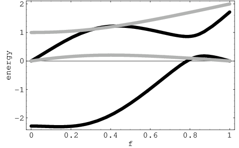
An important caveat in applying this result to quantum algorithms is that while suffices to ensure closely follows the evolution of an eigenvector of , this evolution may not lead to the desired eigenvector of , i.e., corresponding to solutions to the search problem. This is because the eigenvalues of lie on the unit circle in the complex plane and can “wrap around” as increases. Hence, in addition to ensuring the eigenvalue gap does not get too small, good performance also requires selecting appropriate . Alternatively, one could start from a different eigenvector of , which would be useful if one could determine which eigenvector maps to the solutions.
One guarantee of avoiding this problem is that none of the eigenvalues of wrap around the unit circle, i.e., , corresponding to the continuous adiabatic limit. Simulations show performance remains good for moderate values of even if does not go to zero, provided is below some threshold value. For hard random 3-SAT problems with , this threshold appears to be somewhat larger than 1.
To illustrate these remarks consider the example
so . Fig. 6 shows the behavior of the two eigenvalues of for two values of . For the initial ground state eigenvector, with eigenvalue 1, evolves into the eigenvector of rather than the eigenvector corresponding to the ground state of .
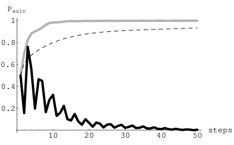
Fig. 7 shows the consequence of this behavior: when is too large, follows the evolving eigenvector to the wrong state when , giving as . As another observation from this figure, exhibits oscillations (though they are quite small for ). With appropriate phase choices, these oscillations can be quite large, allowing to approach 1 with only a modest number of steps, even when approaches 0 for larger . This observation is the basis of the heuristic method.

To see the consequence of this behavior for search, Fig. 8 compares the behavior of several search methods. In this case is sufficiently large that the initial eigenstate of the unitary operator evolves into a nonsolution eigenstate. Thus as the number of steps increases, the probability to find a solution goes to zero, as with the large case in Fig. 7. Nevertheless, for smaller , most of the amplitude “crosses” the gap to another eigenstate that does evolve to a solution state. Consequently, this discrete adiabatic method gives lower overall search cost, using a moderate number of steps, than the continuous adiabatic method (which has as ). By contrast, for larger than 2 or so always remains small.
References
- [1] D. Deutsch. Quantum theory, the Church-Turing principle and the universal quantum computer. Proc. R. Soc. London A, 400:97–117, 1985.
- [2] David P. DiVincenzo. Quantum computation. Science, 270:255–261, 1995.
- [3] Richard P. Feynman. Feynman Lectures on Computation. Addison-Wesley, Reading, MA, 1996.
- [4] Andrew Steane. Quantum computing. Reports on Progress in Physics, 61:117–173, 1998.
- [5] M. R. Garey and D. S. Johnson. Computers and Intractability: A Guide to the Theory of NP-Completeness. W. H. Freeman, San Francisco, 1979.
- [6] Charles H. Bennett, Ethan Bernstein, Gilles Brassard, and Umesh V. Vazirani. Strengths and weaknesses of quantum computing. SIAM Journal on Computing, 26:1510–1523, 1997.
- [7] Edward Farhi et al. A quantum adiabatic evolution algorithm applied to random instances of an NP-complete problem. Science, 292:472–476, 2001.
- [8] V. N. Smelyanskiy, U. V. Toussaint, and D. A. Timucin. Simulations of the adiabatic quantum optimization for the set partition problem. Los Alamos preprint quant-ph/0112143, 2002.
- [9] Giuseppe E. Santoro et al. Theory of quantum annealing of an Ising spin glass. Science, 295:2427–2430, 2002.
- [10] Peter Cheeseman, Bob Kanefsky, and William M. Taylor. Where the really hard problems are. In J. Mylopoulos and R. Reiter, editors, Proceedings of IJCAI91, pages 331–337, San Mateo, CA, 1991. Morgan Kaufmann.
- [11] Scott Kirkpatrick and Bart Selman. Critical behavior in the satisfiability of random boolean expressions. Science, 264:1297–1301, 1994.
- [12] Tad Hogg, Bernardo A. Huberman, and Colin P. Williams, editors. Frontiers in Problem Solving: Phase Transitions and Complexity, volume 81, Amsterdam, 1996. Elsevier. Special issue of Artificial Intelligence.
- [13] Remi Monasson, Riccardo Zecchina, Scott Kirkpatrick, Bart Selman, and Lidror Troyansky. Determining computational complexity from characteristic “phase transitions”. Nature, 400:133–137, 1999.
- [14] Edward Farhi, Jeffrey Goldstone, Sam Gutmann, and Michael Sipser. Quantum computation by adiabatic evolution. Technical Report MIT-CTP-2936, MIT, Jan. 2000.
- [15] Wim van Dam, Michele Mosca, and Umesh Vazirani. How powerful is adiabatic quantum computation? In Proc. of the 42nd Annual Symposium on Foundations of Computer Science (FOCS2001), pages 279–287. IEEE, 2001.
- [16] Tad Hogg. Quantum search heuristics. Physical Review A, 61:052311, 2000. Preprint at publish.aps.org/eprint/gateway/eplist/aps1999oct19_002.
- [17] Tad Hogg. Solving random satisfiability problems with quantum computers. Los Alamos preprint quant-ph/0104048, 2001.
- [18] George W. Snedecor and William G. Cochran. Statistical Methods. Iowa State Univ. Press, Ames, Iowa, 6th edition, 1967.
- [19] R. B. Lehoucq, D. C. Sorensen, and C. Yang. ARPACK User’s Guide: Solution of Large-Scale Eigenvalue Problems with Implicitly Restarted Arnoldi Methods. SIAM, Philadelphia, 1998.
- [20] Bart Selman, Hector Levesque, and David Mitchell. A new method for solving hard satisfiability problems. In Proc. of the 10th Natl. Conf. on Artificial Intelligence (AAAI92), pages 440–446, Menlo Park, CA, 1992. AAAI Press.
- [21] J. Frank, P. Cheeseman, and J. Stutz. When gravity fails: Local search topology. J. of Artificial Intelligence Research, 7:249–281, 1997.
- [22] Jeremie Roland and Nicolas J. Cerf. Quantum search by local adiabatic evolution. Physical Review A, 65:042308, 2002. Los Alamos preprint quant-ph/0107015.
- [23] S. F. Edwards and Raymund C. Jones. The eigenvalue spectrum of a large symmetric random matrix. J. Phys. A: Math. Gen., 9(10):1595–1603, 1976.
- [24] Z. Furedi and K. Komlos. The eigenvalues of random symmetric matrices. Combinatorica, 1:233–241, 1981.
- [25] J. K. L. MacDonald. Successive approximations by the Rayleigh-Ritz variation method. Physical Review, 43:830–833, 1933.
- [26] Per-Olov Lowdin. Studies in perturbation theory: Lower bounds to energy eigenvalues in perturbation-theory ground state. Physical Review, 139:A357–A372, 1965.
- [27] Lov K. Grover. Quantum mechanics helps in searching for a needle in a haystack. Physical Review Letters, 79:325–328, 1997. Los Alamos preprint quant-ph/9706033.
- [28] Michel Boyer, Gilles Brassard, Peter Hoyer, and Alain Tapp. Tight bounds on quantum searching. In T. Toffoli et al., editors, Proc. of the Workshop on Physics and Computation (PhysComp96), pages 36–43, Cambridge, MA, 1996. New England Complex Systems Institute.
- [29] Gilles Brassard, Peter Hoyer, and Alain Tapp. Quantum counting. In K. Larsen, editor, Proc. of 25th Intl. Colloquium on Automata, Languages, and Programming (ICALP98), pages 820–831, Berlin, 1998. Springer. Los Alamos preprint quant-ph/9805082.
- [30] Sebastian M. Maurer, Tad Hogg, and Bernardo A. Huberman. Portfolios of quantum algorithms. Physical Review Letters, 87:257901, 2001. Los Alamos preprint quant-ph/0105071.