Tailoring teleportation to the quantum alphabet
Abstract
We introduce a refinement of the standard continuous variable teleportation measurement and displacement strategies. This refinement makes use of prior knowledge about the target state and the partial information carried by the classical channel when entanglement is non-maximal. This gives an improvement in the output quality of the protocol. The strategies we introduce could be used in current continuous variable teleportation experiments.
pacs
03.67.HkI Introduction
Quantum teleportation has become a cornerstone of quantum information theory since its conception by Bennett et al. in 1993 Bennett et al. 1993. It is a useful quantum information processing task both in itself, and as part of other tasks such as quantum gate implementation Gottesman and Chuang 1999; Knill et al. 2001. In particular, optical implementations of teleportation Bouwmeester et al. 1997; Furusawa et al. 1998; Boschi et al. 1998; Bowen et al. 2002 may be useful in current linear optical quantum computing proposals Knill et al. 2001.
Quantum teleportation is a process whereby the state of a quantum system can be communicated between two (possibly very distant) parties with prior shared entanglement, joint local quantum measurements, local unitary transformations and classical communication. In the standard scheme, the two parties are called Alice and Bob, and are sender and receiver respectively. Victor (the verifier) gives Alice a quantum system (the target) in a state known only to him. Alice makes joint quantum measurements on the target state and her part of the entanglement resource shared with Bob. The results of these measurements she shares with Bob via a classical communication channel. This information tells Bob the local unitary transformations he must perform on his part of the entanglement resource to faithfully reproduce the target at his location. Victor then compares the output state at Bob’s location with the target state by calculating the overlap between the two. In its simplest form this is just the inner product of the two states and is in general known as the fidelity.
In ideal teleportation the resource is maximally entangled. As a result the classical channel carries no information about the target state. Also the alphabet of input states is assumed to be an unbiased distribution over the same dimensions as the entanglement. Examples of this include: the standard discrete protocol where qubits are both the target and entanglement resource Bennett et al. 1993; and the original continuous variable protocol where the target is a flat, infinite dimensional distribution and the entanglement is idealised EPR statesVaidman 1994. However, one may consider situations in which the entanglement is non-maximal and the alphabet of states is not evenly distributed. Additional information is now available prior to teleportation, from the restricted alphabet, and dynamically from the partial target information now carried by the classical channel. How should one then tailor the protocol so as to make best use of this additional information? We address this question in this paper.
The situation arises naturally in practical implementations of continuous variable teleportation Braunstein and Kimble 1998; Ralph and Lam 1998; Furusawa et al. 1998. The entanglement resource most commonly used in continuous variable teleportation is the two-mode squeezed vacuum. It is not perfectly entangled, since this would require infinite energy. On the other hand an even distribution of target states is also unphysical. We are motivated to find ways in which to make maximum use of the resource given this situation. In this paper we outline a general strategy and then describe a simple refinement of the standard continuous variable teleportation protocol which gives an improved output quality for a reduced alphabet of possible input states. It has the advantage that it may be implemented with currently available technology.
Consider the situation of teleporting a coherent state. The state amplitudes will have an upper bound, and the probability of Victor preparing a state with a certain amplitude might be known. Let us consider three variations on this theme:
- Two-dimensional Gaussian.
-
The classical limit used in and derived by Braunstein, Fuchs and Kimble Braunstein et al. 2000 assumes that Victor produces coherent states with a symmetric two-dimensional Gaussian probability distribution, where coherent states of greater amplitude are less likely to occur than those with amplitude close to zero. The standard protocol assumes the width of this distribution is infinite. Braunstein, Fuchs and Kimble considered how the classical limit changed for finite width but not how to optimise the protocol as a function of this width. Choosing this smaller subset of states should allow Alice and Bob to improve the fidelity of their teleportation protocol.
- Coherent states on a circle.
-
Another possibility is that Victor could produce coherent states of an amplitude known to Alice and Bob, but of an unknown phase. If the amplitude of Victor’s prepared coherent states is , then these states will lie on a circle in phase space of radius , hence the term “coherent states on a circle”. This knowledge reduces the alphabet of possible output states substantially and should lead to a corresponding improvement in the fidelity.
- Coherent states on a line.
-
Conversely to coherent states on a circle, Victor could produce target states of known phase but unknown amplitude. These states would lie along a line in phase space and hence are termed “coherent states on a line”. Again, the alphabet of states is reduced and the fidelity is expected to increase with respect to the standard protocol.
II Tailored displacement strategy
We now describe a general strategy for tailoring teleportation based upon maximising the fidelity over Bob’s possible displacements in phase space. Another technique of fidelity optimisation has been discussed by Ide et al. Ide et al. 2002, which uses gain tuning to improve the fidelity output. Our scheme is similar, however we use the one-shot fidelity of teleporting a coherent state to find Bob’s optimum displacement. The technique described here gives very simple relations describing the displacement Bob must make to achieve the best possible fidelity given the level of squeezing, Alice’s measurement results, and the known properties of the target state. Using the transfer operator technique of Hofmann et al. Hofmann et al. 2000, the one-shot fidelity for teleportation of a coherent state is 11 1 The average fidelity is the one-shot fidelity averaged over all measurement results .
| (1) |
where is a parameter combining Alice’s measurement results of position-difference and momentum-sum , is the squeezing parameter and is the displacement to be made by Bob. The variable is determined from Alice’s measurement results and the prior knowledge about the target state. The value of is therefore a “best guess” of the target given the information at hand.
Maximising the fidelity over finds the displacement Bob should make on his mode to give the best reproduction of the target state at his location. The value of which maximises the fidelity is
| (2) |
This has a simple physical interpretation. In the limit of low squeezing, the first term dominates and it is best to use whatever “best guess” we can make for . As the level of squeezing increases, Alice’s measurements () become more relevant and the best guess has less importance. In the limit of large squeezing the first term is negligible in comparison to the second term and we are effectively performing standard continuous variable teleportation.
To illustrate this result, we consider teleportation of states on a line. These are simpler to implement experimentally than states on a circle, since dynamically coordinating the angle of displacement is more difficult than deciding the size of displacement. Hence in this paper we concentrate on states on a line. We know that the states lie along the real axis in phase space, therefore , and is determined from information gathered in the teleportation experiment 22 2 We use the subscripts and to refer to the - and -components respectively of the variables , , and in phase space. Alice’s measurement result gives this information and we set . The relations for the - and -components of the displacement Bob must make are now
| (3) |
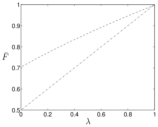
Using this technique results in the dashed curve of Fig. 1, where we observe a significant increase in fidelity over the standard protocol (dot-dashed curve).
III Tailored measurement and displacement strategy
The relations of Eq. (3) tailor only the displacement made by Bob. A further improvement can be obtained if one tailors both the measurements made by Alice and Bob’s displacement. It is easier to perform the calculation in the Heisenberg picture, hence we continue within this formalism. Consider the following situation: Alice and Bob know that they are attempting to teleport coherent states, and they are very sure of the phase of the states, however the input amplitude is unknown. What is the best strategy Alice and Bob can take given that they know the phase of the input state and the level of squeezing? The answer is to tailor Alice’s measurements and Bob’s displacement to the known amount of squeezing. Bob then merely displaces his component of the entanglement resource in the known direction by an amount related to the information sent to him.

The protocol is described diagrammatically in Fig. 2 and proceeds as follows: Alice and Bob share one part of a two-mode squeezed vacuum generated by parametric down conversion of the vacua and in the squeezer denoted SQ in the figure. Once again the phase of the target coherent state is taken to be zero. We do not lose generality since it is always possible to rotate to a frame in which the phase of the target state points along the real axis in phase space. Alice mixes her mode with that of the target state on a beam splitter. The level of mixing is varied by choosing the beam splitter reflectance in a manner dependent upon the level of squeezing . Alice makes measurements of the quadrature observables and , which are given by
| (4) | ||||
| and | ||||
| (5) | ||||
Note that for a general mode the quadrature components are given by
| (6) |
These she modifies by the gain parameters and respectively before sending this information to Bob via a classical channel. The parameters and are dependent upon the level of squeezing and the beam splitter reflectance. Bob uses this information to displace his mode along the real axis and obtain an approximate reproduction of the initial target state.
The output field from the protocol is
| (7) |
from which it is possible show that the quadrature amplitudes of are
| (8) | ||||
| (9) |
Note that normalisation factors have been absorbed into the gains and . This means that at unit gain, when the output mode is described by
| (10) |
the gains are instead of , as for other conventions.
Assuming our states are uniformly distributed along the line (out to some large ) then unit gain for the real quadrature is the best strategy (as in standard teleportation). We can determine from this constraint and so we choose
| (11) |
This value for gives the new amplitude quadrature of the output mode as
| (12) |
Unlike the standard protocol, we know that the average value of the phase quadrature is zero. Thus we are free to choose the gain on the phase quadrature, , such that it maximises the fidelity. The amplitude and phase quadrature variances of are
| (13) | ||||
| (14) |
These values are then substituted into the average fidelity at unit gain Furusawa et al. 1998
| (15) |
which we now maximise over . Maximising the fidelity is equivalent to minimising the phase quadrature variance over the same variable. Performing this minimisation gives the new value of
| (16) |
and the protocol is tailored for states on a line.
Let us consider various limits of the protocol, and measurement and displacement strategies at those limits. When there is no squeezing, one should just measure the amplitude of the incoming state since its phase is known. This situation is represented in our protocol by using a completely transmissive beam splitter and ignoring the measurement. The parameters in this situation are therefore (completely transmissive beam splitter), (no squeezing), and (ignoring all information measured in the quadrature). This situation gives an amplitude quadrature variance of and a phase quadrature variance of , and hence a fidelity of . Performing standard teleportation at unit gain with no squeezing gives a fidelity of Braunstein and Kimble 1998; Braunstein et al. 2000. One can therefore see that our protocol gives a good improvement over standard techniques. If we choose to teleport using a 50:50 beam splitter we recover the result for only tailoring the displacement. With no squeezing, again the best thing to do is ignore the phase quadrature. This gives the parameter values (50:50 beam splitter), and . However, since we are mixing in half of the unsqueezed vacuum, we introduce an extra noise component, increasing the amplitude quadrature variance to with the phase quadrature variance being the same at ; now the fidelity is . For large amounts of squeezing , and it is best to use a 50:50 beam splitter and perform standard teleportation. In this limit the quadrature variances become and respectively, and the fidelity tends to unity.

In Fig. 3 we show these limits graphically and the trends of three teleportation protocols as a function of squeezing parameter . The solid line represents the average fidelity as a function of squeezing for the tailored measurement and displacement scheme. As mentioned above it starts at at no squeezing () and tends to unity as the level of squeezing increases. Note that this is a marked improvement over the standard protocol as shown by the dot-dashed curve. The dashed curve is the fidelity function when Alice’s beam splitter is set at 50:50, resulting in no tailored measurement, but still using tailored displacement. The fidelity begins at and tends to unity with increasing squeezing. This too is a good improvement over the standard protocol.

In order to obtain tailored measurement and displacement average fidelity as a function of squeezing, one must maximise the fidelity over both the phase quadrature gain and the beam splitter parameter . The gain and beam splitter parameter values as functions of squeezing parameter are shown in Fig. 4. The gain (solid curve) increases smoothly from zero at no squeezing and tends to at infinite squeezing (). The limits are expected since at no squeezing one does not want to include any information from the phase quadrature measurement, and hence the gain should be zero. The large squeezing limit also makes sense since for large squeezing the teleporter should be at unit gain, which corresponds to a value of . The beam splitter parameter (dashed curve) begins at zero at no squeezing and increases smoothly to (note that is given in units of in Fig. 4). Again, this is sensible behaviour: at no squeezing one should just measure the target without mixing in any of the squeezed beam . To do this one should have a completely transmissive beam splitter, which is when . At infinite squeezing one should equally mix the target and Alice’s half of the entanglement resource. So, one should use a 50:50 beam splitter, which corresponds to a beam splitter parameter value of .
The tailored displacement only strategy curve of Fig. 1 calculated from Eq. (2) is identical to the equivalent curve in Fig. 3 showing the consistency of the two approaches. It also turns out, for sufficiently large, that using the tailored displacement scheme to teleport coherent states “on a circle” gives the same fidelity versus squeezing parameter relationship as that found for teleporting coherent states on a line. Bob’s displacement in this instance has - and -components
| (17) | ||||
| (18) |
where and are the best guesses for and respectively, and . This result is supported by the paper of Ide et al. Ide et al. 2002 where they too discussed the optimal teleportation of coherent states of known amplitude, but unknown phase and showed an average fidelity versus squeezing parameter relationship very similar to that shown in Fig. 1 of this paper. That states on a line and states on a circle have the same fidelity relationship indicates that the two situations are interchangeable; the trends from one can be used to give the results for the other. Further improvement of teleportation for states on the circle would require the use of adaptive phase measurements Wiseman 1995.
IV Two-dimensional distributions in phase space
We now adapt the tailored displacement scheme in the Heisenberg picture to the situation of the target state alphabet being a two-dimensional distribution in phase space. Let’s begin by deriving the fidelity of teleportation for a variable linear gain applied to both Alice’s measurement results, and a target field mixed with Alice’s part of the two-mode squeezed vacuum entanglement resource on a 50:50 beam splitter. To do this we calculate the variance of the teleporter output field . For a level of squeezing , the output field amplitude quadrature can be shown to be
| (19) |
where and are the vacua prior to being squeezed in the parametric down converter. This is the same situation as in Fig. 2 where and . It is possible to show that the variance of this quadrature is
| (20) |
The phase quadrature and its corresponding variance are equal to and respectively. This is now sufficient information to calculate the average fidelity, which for a general gain has the form Furusawa et al. 1998
| (21) |
where is the amplitude of the coherent state being teleported, and is the phase quadrature variance.
To make use of the knowledge of the target state alphabet, we weight this fidelity by the probability of Victor preparing a given target state . A simple case of this probability is a two-dimensional Gaussian distribution centred at the origin in phase space. This form of the distribution will be used in the following discussion since it was used by Braunstein, Fuchs and Kimble Braunstein et al. 2000, hence their results can be compared with those presented here.
The probability of Victor preparing a given state in phase space is given by
| (22) |
where and are the standard deviations of the Gaussian in the - and -directions respectively. An overall figure of merit for the teleportation protocol is the optimised average fidelity defined by
| (23) |
where the integral is taken over all possible values of . Notice that the optimised average fidelity is an implicit function of the gain , and the amount of squeezing . In the examples that follow, this optimised average fidelity is numerically maximised over the gain to find the relationship between the average fidelity and the level of squeezing, , for the given alphabet of target states.
Let’s now look at two examples of probability distributions in phase space. We shall initially analyse a symmetric Gaussian with very large standard deviation, the reason being that this example corresponds well with standard continuous variable teleportation. We will then investigate a very narrow symmetric distribution and compare the no squeezing limit with the classical level derived by Braunstein, Fuchs and Kimble.
In the first example, the distribution is symmetric with standard deviation . Such a distribution is a very good approximation of the situation in standard continuous variable teleportation, where it is assumed that the alphabet of target states is a flat distribution over all phase space. Calculating the optimised average fidelity maximised over the gain as a function of squeezing parameter one obtains the trend in Fig. 5.
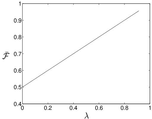
The optimised average fidelity increases linearly from at no squeezing to at infinite squeezing. This is the same curve as the dot-dashed curve in Fig. 3. This result is expected since, as mentioned above, a very broad Gaussian distribution is a good approximation to the perfectly flat distribution of target states assumed in the standard protocol.
In the second example, the distribution is symmetric with standard deviation . This is a very narrow distribution and one would expect to find a high optimised average fidelity for all levels of squeezing since the alphabet of target states does not deviate far from the vacuum. Performing tailored displacement teleportation using this distribution as the alphabet of target states and maximising the optimised average fidelity over the gain, one produces the optimised average fidelity versus squeezing parameter relationship shown in Fig. 6.
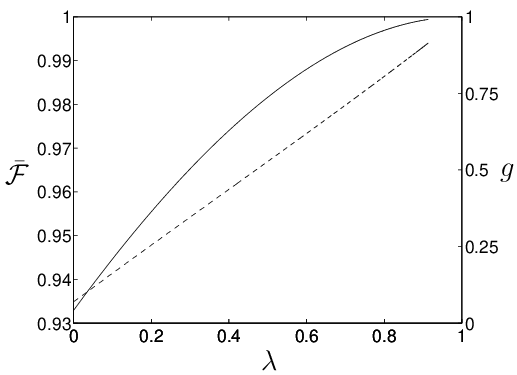
Note that the optimised average fidelity at (i.e. the classical level) is very much greater than the value of normally predicted by standard teleportation. Braunstein, Fuchs and Kimble Braunstein et al. 2000 derived a relationship between the average fidelity at the classical limit and the spread of the two-dimensional Gaussian, optimised for the given distribution. This relationship is
| (24) |
where is inversely proportional to the square of the standard deviation of the Gaussian. In the discussion here where . For a symmetric Gaussian of standard deviation , using Eq. (24) one would expect the optimised average fidelity at the classical level to be . At in Fig. 6 one finds that . A similar level of agreement exists for all values of the standard deviation . Thus, to a good approximation, our results agree with the classical limit of Braunstein, Fuchs and Kimble.
Overall, one can still make use of the prior knowledge of the target state alphabet and optimise the protocol over the gain for nonzero levels of squeezing. This is what has been done here; the fidelity increases from the classical level up to unity with increasing squeezing as shown explicitly in Fig. 6. The tailored displacement teleportation technique again being useful in improving continuous variable teleportation.
V Summary
We have introduced a refined measurement and displacement strategy which makes good use of the properties of prior knowledge about the target state and non-maximal entanglement. This refinement is tailored to the given experimental situation and shown to give a great improvement on the output quality of continuous variable teleportation. The two techniques of calculating the tailored displacement strategy gave identical results, and some physical insight into how this strategy works.
We also analysed symmetric two-dimensional Gaussian distributions of coherent states as an alphabet of target states. We showed agreement with the results of Braunstein, Fuchs and Kimble, and extended their work by including squeezing in the model.
The strategy described here is generally applicable to all teleportation schemes involving physically limited resources. A major advantage of this scheme is that it is able to be implemented with current continuous variable teleportation technology since it only requires linear gain on the measurement results.
Acknowledgements.
PTC acknowledges the financial support of the Centre for Laser Science, the University of Queensland and the Australian Research Council. The authors thank G. J. Milburn for helpful discussions and insights in the production of this work.References
- Bennett et al. (1993) C. H. Bennett, G. Brassard, C. Crepeau, R. Jozsa, A. Peres, and W. K. Wootters, Phys. Rev. Lett. 70(13), 1895 (1993).
- Gottesman and Chuang (1999) D. Gottesman and I. L. Chuang, Nature 402, 390 (1999).
- Knill et al. (2001) E. Knill, R. Laflamme, and G. J. Milburn, Nature 409, 46 (2001).
- Bouwmeester et al. (1997) D. Bouwmeester, J.-W. Pan, K. Mattle, M. Eibl, H. Weinfurter, and A. Zeilinger, Nature 390, 575 (1997).
- Furusawa et al. (1998) A. Furusawa, J. L. Sorensen, S. L. Braunstein, C. A. Fuchs, H. J. Kimble, and E. S. Polzik, Science 282, 706 (1998).
- Boschi et al. (1998) D. Boschi, S. Branca, F. D. Martini, L. Hardy, and S. Popescu, Phys. Rev. Lett. 80(6), 1121 (1998).
- Bowen et al. (2002) W. P. Bowen, N. Treps, B. C. Buchler, R. Schnabel, T. C. Ralph, H. A. Bachor, T. Symul, and P. K. Lam, Experimental investigation of continuous variable quantum teleportation (2002), quant-ph/0207179.
- Vaidman (1994) L. Vaidman, Phys. Rev. A 49(2), 1473 (1994).
- Braunstein and Kimble (1998) S. L. Braunstein and H. J. Kimble, Phys. Rev. Lett. 80(4), 869 (1998).
- Ralph and Lam (1998) T. C. Ralph and P. K. Lam, Phys. Rev. Lett. 81(25), 5668 (1998).
- Braunstein et al. (2000) S. L. Braunstein, C. A. Fuchs, and H. J. Kimble, Journal of Modern Optics 47(2/3), 267 (2000).
- Ide et al. (2002) T. Ide, H. F. Hofmann, A. Furusawa, and T. Kobayashi, Phys. Rev. A 65, 062303 (2002).
- Hofmann et al. (2000) H. F. Hofmann, T. Ide, T. Kobayashi, and A. Furusawa, Phys. Rev. A 62, 062304 (2000).
- Wiseman (1995) H. M. Wiseman, Phys. Rev. Lett. 75(25), 4587 (1995).