Entanglement Properties of the Harmonic Chain

K. Audenaert Email: k.audenaert@ic.ac.uk Affiliation: QOLS, Blackett Laboratory, Imperial College of Science, Technology and Medicine, London, SW7 2BW, UK J. Eisert Email: j.eisert@ic.ac.uk Affiliation: QOLS, Blackett Laboratory, Imperial College of Science, Technology and Medicine, London, SW7 2BW, UK M.B. Plenio Email: m.plenio@ic.ac.uk Affiliation: QOLS, Blackett Laboratory, Imperial College of Science, Technology and Medicine, London, SW7 2BW, UK R.F. Werner Email: R.Werner@tu-bs.de Affiliation: Institut für Mathematische Physik, TU Braunschweig, Mendelssohnstraße 3, 38106 Braunschweig, Germany

August 11, 2026

Abstract

We study the entanglement properties of a closed chain of harmonic oscillators that are coupled via a translationally invariant Hamiltonian, where the coupling acts only on the position operators. We consider the ground state and thermal states of this system, which are Gaussian states. The entanglement properties of these states can be completely characterized analytically when one uses the logarithmic negativity as a measure of entanglement.

pacs

03.67.-a, 03.67.Hk

I Introduction

Quantum entanglement is possibly the most intriguing property of states of composite quantum systems. It manifests itself in correlations of measurement outcomes that are stronger than attainable in any classical system. The renewed interest in a general theory of entanglement in recent years is largely due to the fact that entanglement is conceived as the key resource in protocols for quantum information processing. Initial investigations focused on the properties of bipartite entanglement of finite dimensional systems such as two-level systems. In fact, significant progress has been made, and our understanding of the entanglement of such systems is quite well developed Entanglement. A natural next step is the extension of these investigations to multi-partite systems. Unfortunately, the study of multi-partite entanglement suffers from a proliferation of different types of entanglement already in the pure state case MREGS, and even less is known about the mixed state case. For example, necessary and sufficient criteria for separability are still lacking. For other properties, such as distillability, no efficient decision methods are known, and it is even difficult to find meaningful entanglement measures Jens+Martin. A direction that promises to lead to simpler structures is that of infinite dimensional subsystems, such as harmonic oscillators or light modes, which are commonly denoted as continuous-variable systems cvs; cvs2. Indeed, for continuous-variable systems the situation becomes much more transparent if one restricts attention to Gaussian states (e.g. coherent, squeezed or thermal states) which are, in any case, the states that are readily experimentally accessible.

Quite recently, it has been realized that it might be a very fruitful enterprise to apply the methods from the theory of entanglement not only to problems of quantum information science, but also to the study of quantum systems that are typically regarded as belonging to statistical physics, systems that consist of a large or infinite number of coupled subsystems NielsenPhD; Interacting; exact; Bro. Examples of such systems are interacting spin systems, which, like most interacting systems, exhibit the natural occurrence of entanglement, i.e., the ground state is generally an entangled state NielsenPhD; Interacting; exact. It has, furthermore, been suspected that the study of the entanglement properties of such systems may shed light on the nature of the structure of classical and quantum phase transitions NielsenPhD; exact. It has turned out, however, that the theoretical analysis of infinite spin chains is very complicated and only very rare examples can be solved analytically. Coupled harmonic oscillator systems allow for a much better mathematical description of their entanglement properties than spin systems. Physical realizations of such systems range from the vibrational degrees of freedom in lattices to the discrete version of free fields in quantum field theory. This motivates the approach that we have taken in this work, namely to investigate the entanglement structure of infinitely extended harmonic oscillator systems.

In this paper we study a special case, namely a set of harmonic oscillators arranged on a ring and furnished with a harmonic nearest-neighbor interaction, i.e., oscillators that are connected to each other via springs. The paper is organized as follows. In Section II we provide the basic mathematical tools that are employed in the analysis following in the remaining sections. We then move on to derive a simple analytical expression for the ground state energy of the harmonic oscillator systems. Our main interest is the computation of entanglement properties of the ground state of the chain. In Section III we derive a general formula for the logarithmic negativity Nega; Mono which we employ as our measure of entanglement. In Section IV we present analytical results that concern the symmetrically bisected chain, that is the situation where the chain is subdivided into two equal contiguous parts and the entanglement is calculated between those parts. We show how to construct a very simple lower bound on the log-negativity, in the form of a closed-form expression based on the coupling strengths; that is, no matrix calculations are necessary. Furthermore, for nearest-neighbor interaction, we show that the bound is sharp, i.e., gives the exact value of the log-negativity. Surprisingly, the value of the log-negativity in this case is independent of the chain length; in particular, it remains finite. We show in Section V that the problem is not reducible to a four-oscillator picture, thereby demonstrating the non-triviality of the physical system. We then move on to Section VI, where we study general bisections of the chain numerically. We demonstrate that entanglement is maximized for the symmetrically bisected chain. Furthermore, and rather counterintuitively, for asymmetric bisections where one group of oscillators is very small, and especially when it consists of only one oscillator, we find that the entanglement decreases if the size of the other group is increased. We also demonstrate that for large numbers of oscillators the mean energy of the ground state and the value of the negativity are proportional and provide an interpretation for this result. In Section VII we discuss our results. We also provide an intuitive picture that allows to explain the results in the previous sections.

Generally we have attempted to structure the sometimes somewhat involved mathematics in such a way, that the reader can skip it and extract the main physical results easily. We state at the beginning of each section what main result will be obtained and we state this result clearly, either in the form of a theorem or at the end of the section.

II Covariance matrix for Gaussian states of the harmonic chain

In this section we derive an expression for the covariance matrix of the ground state and of the thermal states of a set of harmonic oscillators that are coupled via a general interaction that is quadratic in the position operators (e.g. oscillators coupled by springs). As a byproduct we also give an expression for the energy of the ground state.

Let us first consider the covariance matrix for the ground state of a single uncoupled harmonic oscillator. The Hamiltonian is given by (we have adopted units where $\hbar=1$ )

\hat{H}=\frac{1}{2m}\hat{P}^{2}+\frac{m\omega^{2}}{2}\hat{X}^{2}.

Denoting the quadrature operators as a column vector $R$ , with $R_{1}=\hat{X}$ and $R_{2}=\hat{P}$ , the Hamiltonian can be concisely rewritten as

\hat{H}=R^{T}\left(\begin{array}[]{cc}m\omega^{2}/2&0\\ 0&1/(2m)\end{array}\right)R.

The covariance matrix $\gamma$ of a general state $\rho$ is given by

\gamma_{k,l}=\text{Re }{\mathrm{T}r}[\rho(R_{k}-{\mathrm{T}r}[\rho R_{k}])(R_{l}-{\mathrm{T}r}[\rho R_{l}])].

for $1\leq k,l\leq 2$ . For $\rho_{n}$ the $n$ -th eigenstate of the Hamiltonian, $\rho_{n}=|n\rangle\langle n|$ , it is a straightforward exercise to calculate that

\gamma=(n+1/2)\left(\begin{array}[]{cc}1/(m\omega)&0\\ 0&m\omega\end{array}\right).

We will only be interested in the ground state, $\rho_{0}=|0\rangle\langle 0|$ , however, since this is the only eigenstate which is Gaussian.

Passing to the harmonic chain consisting of $n$ harmonic oscillators, we will only consider interactions between the oscillators due to a coupling between the different position operators. According to the $(q,p)$ -convention we have adopted here, the vector $R$ of quadrature operators is given by $R_{j}=\hat{X}_{j}$ and $R_{n+j}=\hat{P}_{j}$ , for $1\leq j\leq n$ . The Hamiltonian is then of the form

\hat{H}=R^{T}\left(\begin{array}[]{cc}Vm\omega^{2}/2&0\\ 0&\openone_{n}/(2m)\end{array}\right)R,

where the $n\times n$ -matrix $V$ contains the coupling coefficients. The Hamiltonian is thus written as a quadratic form in the quadrature operators; we will call the matrix corresponding to this form the Hamiltonian matrix (as opposed to $\hat{H}$ , the Hamiltonian operator). In the present case, the Hamiltonian matrix is a direct sum of the kinetic matrix $\openone_{n}/(2m)$ and the potential matrix $Vm\omega^{2}/2$ .

In this paper, we will consider a harmonic chain “connected” end-to-end by a translationally invariant Hamiltonian. The $V$ -matrix of the Hamiltonian is, therefore, a so-called circulant matrix HJ2. This is a special case of a Toeplitz matrix because not only do we have $V_{j,k}=v_{j-k}$ , but even $V_{j,k}=v_{(j-k)\bmod n}$ for $1\leq j,k\leq n$ , due to the end-to-end connection. We can easily write the coefficients $v_{k}$ in terms of the coupling coefficients. For a nearest-neighbor coupling with “spring constant” $K$ , the potential term of the Hamiltonian reads

\sum_{k=1}^{n}\frac{m\omega^{2}}{2}\hat{X}_{k}^{2}+K(\hat{X}_{(k+1)\bmod n}-\hat{X}_{k})^{2}.

Therefore, we have

v_{0}=1+4K/(m\omega^{2}),\,\,\,v_{1}=-2K/(m\omega^{2}).

More generally, including $k$ -th nearest-neighbor couplings with spring constants $K_{k}$ , and defining

\alpha_{k}=\frac{2K_{k}}{m\omega^{2}},

we have

	$\displaystyle v_{0}$	$\displaystyle=$	$\displaystyle 1+2(\alpha_{1}+\alpha_{2}+\ldots),$
	$\displaystyle v_{j}$	$\displaystyle=$	$\displaystyle-\alpha_{j},\text{ for }j>0.$

The calculation of the corresponding covariance matrix can now proceed via a diagonalisation of the Hamiltonian matrix, which effectively results in a decoupling of oscillators. Since the commutation relations between the quadrature operators must be preserved, the diagonalisation must be based on a symplectic transformation $S\in Sp(2n,{\mathbb{R}})$ . This means that we can only use equivalence transformations $C\mapsto C^{\prime}=S^{T}CS$ such that $S^{T}\Sigma S=\Sigma$ , where, in the $(q,p)$ -convention, the symplectic matrix $\Sigma$ is given by

\Sigma=\left(\begin{array}[]{cc}0&\openone_{n}\\ -\openone_{n}&0\end{array}\right).

This real skew-symmetric matrix incorporates the canonical commutation relations between the canonical coordinates. Fortunately, because the kinetic matrix is a multiple of the identity, the Hamiltonian matrix can be diagonalized by an orthogonal equivalence of the form

C\longmapsto C^{\prime}=(S\oplus S)^{T}C(S\oplus S),

where $S$ is the real orthogonal $n\times n$ -matrix that diagonalizes the potential matrix $V$ . It is readily checked that the resulting transformation is indeed a symplectic one. In fact, $S\oplus S$ is an element of the maximal compact subgroup of $Sp(2n,{\mathbb{R}})$ .

So $C^{\prime}$ is now diagonal and of the form $C^{\prime}=(m\omega^{2}/2)V^{\prime}\oplus\openone_{n}/(2m)$ , where $V^{\prime}$ is the diagonal $n\times n$ -matrix with entries $\eta_{j}$ , $1\leq j\leq n$ , the eigenvalues of $V$ . The covariance matrix $\gamma^{\prime}$ of the ground state of the transformed Hamiltonian consists therefore just of single-oscillator covariance matrices with parameter $\omega_{j}=\omega\sqrt{\eta_{j}}$ , $1\leq j\leq n$ , and is diagonal itself, to wit,

$\displaystyle\gamma^{\prime}$	$\displaystyle=$	$\displaystyle(\gamma^{\prime}_{x}\oplus\gamma^{\prime}_{p})/2,$
$\displaystyle(\gamma^{\prime}_{x})_{j,j}$	$\displaystyle=$	$\displaystyle 1/(m\omega_{j}),$
$\displaystyle(\gamma^{\prime}_{p})_{j,j}$	$\displaystyle=$	$\displaystyle m\omega_{j}.$

The covariance matrix $\gamma$ in the original coordinates is then obtained by transforming $\gamma^{\prime}$ back,

$\displaystyle\gamma$	$\displaystyle=$	$\displaystyle(S\oplus S)\gamma^{\prime}(S\oplus S)^{T}$
	$\displaystyle=$	$\displaystyle[(S\gamma^{\prime}_{x}S^{T})\oplus(S\gamma^{\prime}_{p}S^{T})]/2$
	$\displaystyle=$	$\displaystyle[(V^{-1/2}/(m\omega))\oplus(m\omega V^{1/2})]/2.$

To simplify the notation, we will henceforth set $m=1$ and $\omega=1$ . So we have a simple formula for the covariance matrix in terms of the potential matrix $V$ ,

$\displaystyle\gamma$	$\displaystyle=$	$\displaystyle(\gamma_{x}\oplus\gamma_{p})/2,$
$\displaystyle\gamma_{x}$	$\displaystyle=$	$\displaystyle V^{-1/2},$
$\displaystyle\gamma_{p}$	$\displaystyle=$	$\displaystyle V^{1/2}.$

Using this same derivation, we can also easily find a formula for the energy of the ground state. We will need this result in Section VI, where we will compare the log-negativity of a state to its energy. Indeed, the ground state energy of a single oscillator is $\hbar\omega/2$ . In the decoupled description of the ground state of the chain, the oscillators have energy $\hbar\omega\sqrt{\eta_{j}}/2$ , with $\eta_{j}$ , $1\leq j\leq n$ , being the eigenvalues of the potential matrix $V$ . The total ground state energy is $E=(\hbar\omega/2)\sum_{j=1}^{n}\sqrt{\eta_{j}}$ . Denoting $\hbar\omega/2$ by $E_{0}$ , we therefore have

E=E_{0}{\mathrm{T}r}[V^{1/2}].

Finally, we turn to Gibbs states corresponding to some temperature $T>0$ , the states associated with the canonical ensemble, given by

\rho(\beta)=\exp(-\beta\hat{H})/{\mathrm{T}r}[\exp(-\beta\hat{H})],

where $\beta=1/T$ . Again, one can obtain the covariance matrix $\gamma(\beta)$ of the state $\rho(\beta)$ in a convenient manner in the basis in which the Hamiltonian matrix is diagonal. The $2n\times 2n$ diagonal matrix $\gamma^{\prime}(\beta)$ can be obtained using the virial theorem: the mean potential energy and the kinetic energy of a single oscillator are identical and half the mean energy of the system at inverse temperature $\beta$ . Using this procedure one obtains

$\displaystyle\gamma^{\prime}(\beta)$	$\displaystyle=$	$\displaystyle(\gamma^{\prime}_{x}(\beta)\oplus\gamma^{\prime}_{p}(\beta))/2,$
$\displaystyle(\gamma^{\prime}_{x}(\beta))_{j,j}$	$\displaystyle=$	$\displaystyle\frac{1}{m\omega_{j}}\left(1+\frac{2}{\exp(\beta\omega_{j})-1}\right),$
$\displaystyle(\gamma^{\prime\prime}_{p}(\beta))_{j,j}$	$\displaystyle=$	$\displaystyle m\omega_{j}\left(1+\frac{2}{\exp(\beta\omega_{j})-1}\right).$

In the convention where $m=1$ , $\omega=1$ , one gets

$\displaystyle\gamma(\beta)$	$\displaystyle=$	$\displaystyle(\gamma_{x}(\beta)\oplus\gamma_{p}(\beta))/2,$
$\displaystyle\gamma_{x}(\beta)$	$\displaystyle=$	$\displaystyle V^{-1/2}\Bigl(\openone_{n}+2(\exp(\beta V^{1/2})-\openone_{n})^{-1}\Bigr),$
$\displaystyle\gamma_{p}(\beta)$	$\displaystyle=$	$\displaystyle V^{1/2}\Bigl(\openone_{n}+2(\exp(\beta V^{1/2})-\openone_{n})^{-1}\Bigr),$

for the covariance matrix of a Gibbs state in the original canonical coordinates.

III General formula for the logarithmic negativity

In this section we derive a general formula for the logarithmic negativity of a Gaussian state of $n$ coupled harmonic oscillators with respect to a bipartite split, given the covariance matrix $\gamma$ of the Gaussian state. This set may consist of all $n$ oscillators or of a subset of $m<n$ oscillators. The only restriction is that the covariance matrix must be a direct sum of a position part $\gamma_{x}$ and a momentum part $\gamma_{p}$ , i.e., there must be no correlations between positions and momenta. The resulting formula can be found at the end of this section.

Let $m_{1}$ and $m_{2}$ be the sizes of the two groups of oscillators the entanglement between which we wish to calculate, and let $m=m_{1}+m_{2}\leq n$ . From Section II, we know that the covariance matrix $\gamma$ of the ground state of the harmonic chain is given by $\gamma=(\gamma_{x}\oplus\gamma_{p})/2$ , where $\gamma_{x}=V^{-1/2}$ and $\gamma_{p}=V^{1/2}$ . In order to calculate the entanglement between two disjoint groups of oscillators in this state, we need to consider the covariance matrix associated with the reduced state of the $m$ oscillators of the two groups. This covariance matrix $\mu$ – from now on also referred to as reduced covariance matrix – is given by the $2m\times 2m$ principal submatrix of $\gamma$ that consists of those rows and colums of $\gamma$ that correspond to the canonical coordinates of either group $1$ or group $2$ . If $m=n$ , meaning that the whole set of $n$ oscillators is considered, this step is not necessary. The reduced covariance matrix $\mu$ is again of the form

\mu=(\mu_{x}\oplus\mu_{p})/2,

where both $\mu_{x}$ and $\mu_{p}$ are $m\times m$ -matrices.

Taking the partial transpose of a covariance matrix corresponds to changing the sign of the momentum variables of the oscillators in the second group. This operation maps the covariance matrix $\mu$ to

\mu^{\Gamma}=P\mu P

with

P=P_{x}\oplus P_{p},\,\,\,\,P_{x}=\openone_{m};

$P_{p}$ is a $m\times m$ diagonal matrix. Specifically, the $j$ -th diagonal element of $P_{p}$ is $1$ or $-1$ , depending on whether the oscillator on position $1\leq j\leq m$ belongs to group 1 or 2, respectively.

The logarithmic negativity Nega; Mono of a state is defined as the logarithm of the trace norm of the partial transpose of the state. The negativity is an entanglement measure in the sense that it is a functional that is monotone under local quantum operators Mono; PhD. To date it is the only feasible measure of entanglement for mixed Gaussian quantum states. The definition of the logarithmic negativity can be easily translated into an expression which does not involve the state itself, but rather the covariance matrix of the state: as the trace norm is unitarily invariant, one has the freedom to choose a basis for which the evaluation of the trace norm becomes particularly simple. More specifically, one may make use of the Williamson normal form Wil for the partial transpose of the covariance matrix. The problem of evaluating the logarithmic negativity is then essentially reduced to a single-mode problem. This procedure gives rise to the formula Mono

N=-\sum_{k=1}^{2m}\log_{2}(\min(1,2|{\lambda}_{k}(i\Sigma^{-1}\mu^{\Gamma})|)),

where ${\lambda}_{k}(i\Sigma^{-1}\mu^{\Gamma})$ , $1\leq k\leq 2m$ , are the eigenvalues of $i\Sigma^{-1}\mu^{\Gamma}$ . $\Sigma$ is the symplectic matrix

\Sigma=\left(\begin{array}[]{cc}0&\openone_{m}\\ -\openone_{m}&0\end{array}\right).

Since $\Sigma^{-1}=-\Sigma$ , we have to calculate the spectrum of the matrix $B=-i\Sigma P\mu P$ , giving $2m$ real eigenvalues $\lambda_{k}(B)$ of $B$ . Then the logarithmic negativity equals $N=-\sum_{k=1}^{2m}\log_{2}\min(1,2|\lambda_{k}(B)|)$ . This formula can be further simplified due to the direct sum structure of $\mu=(\mu_{x}\oplus\mu_{p})/2$ . Simplification of $B$ yields

B=\frac{i}{2}\left(\begin{array}[]{cc}0&-P_{p}\mu_{p}P_{p}\\ \mu_{x}&0\end{array}\right).

The eigenvalue equation of a block matrix of this form reads

\left(\begin{array}[]{cc}0&X\\ Y&0\end{array}\right)\left(\begin{array}[]{c}u\\ v\end{array}\right)=\lambda\left(\begin{array}[]{c}u\\ v\end{array}\right),

which is equivalent to the coupled system of equations $Xv=\lambda u$ and $Yu=\lambda v$ . Substituting one equation in the other yields $XYu=\lambda^{2}u$ , hence the eigenvalues of the block matrix are plus and minus the square roots of the eigenvalues of $XY$ . In particular, the eigenvalues of $B$ are $\pm(\lambda_{j}(\mu_{x}P_{p}\mu_{p}P_{p}/4))^{1/2}$ , $1\leq j\leq m$ . Because of the $\pm$ -sign, taking the absolute value of the eigenvalues has the effect of doubling the eigenvalue multiplicity. Hence,

N=-\sum_{j=1}^{m}\log_{2}\min(1,\lambda_{j}(\mu_{x}P_{p}\mu_{p}P_{p})),

which is finally the resulting formula of the logarithmic negativity in terms of the matrices $\mu_{x}$ and $\mu_{p}$ .

IV The Symmetrically Bisected Harmonic Chain

In this section we present exact analytical results for the log-negativity in a chain of $n$ harmonic oscillators with a translationally invariant coupling. Moreover, we shall be interested here in the most symmetric case of calculating the entanglement with respect to a symmetric bisection of the chain. That is, the number $n$ of oscillators should be even and the oscillators in positions 1 to $n/2$ constitute group 1, the others group 2 (see Figure 1). Hence, in the notation of Section III $\mu=\gamma$ .

Refer to caption — Figure 1: The symmetrically bisected harmonic chain. The oscillators $1$ to $n/2$ form group $1$ , the oscillators $n/2+1$ to $n$ form group $2$ .

Using the result of Section III, we find that the logarithmic negativity of a symmetrically bisected oscillator chain, of length $n$ and with potential matrix $V$ , is equal to

N=-\sum_{j=1}^{n}\log_{2}(\min(1,\lambda_{j}(Q))),

with

	$\displaystyle Q$	$\displaystyle=$	$\displaystyle V^{-1/2}PV^{1/2}P$
	$\displaystyle P$	$\displaystyle=$	$\displaystyle\openone_{n/2}\oplus(-\openone_{n/2}).$

IV.1 Symmetry properties of $Q$

We begin our analytical investigations by studying a more general object than $Q$ , namely the matrix

R=G^{-1}PGP.

Here, $G$ is a general real circulant matrix that is symmetric under transposition. Since $G$ is symmetric and circulant, it can be written in $2\times 2$ block form as

G=\left(\begin{array}[]{cc}G^{\prime}&G^{\prime\prime}\\ G^{\prime\prime}&G^{\prime}\end{array}\right).

We will first show that $R$ exhibits the same block structure. Define the $n\times n$ flip-matrix $F=F_{n}$ as

F_{i,j}=\delta_{i,n+1-j}.

To simplify the notation, we will mostly refrain from mentioning the size $n$ of $F$ ; the mathematical context should make it clear which $n$ is being used.

Lemma 1

The matrix $R$ can be written in $2\times 2$ block form as

R=\left(\begin{array}[]{cc}A&B\\ B&A\end{array}\right).

Proof. Since $G$ is circulant and symmetric, $FGF=G$ , which is true for every symmetric Toeplitz matrix. Also, $FPF=-P$ holds. Writing

R=\left(\begin{array}[]{cc}A&B\\ C&D\end{array}\right),

symmetry demands that $C=FBF$ and $D=FAF$ . Furthermore, both $G$ and $P$ are also invariant under the $F_{n/2}\oplus F_{n/2}$ symmetry. Hence, $R$ exhibits this symmetry too, i.e., $(F\oplus F)R(F\oplus F)=R$ . Thus, $A$ and $B$ are invariant under $F$ . $\square$

Matrices with this block structure can be brought in block diagonal form using a similarity transform:

Lemma 2

Let ${\cal S}=(P+F)/\sqrt{2}$ . Then

{\cal S}\left(\begin{array}[]{cc}A&B\\ B&A\end{array}\right){\cal S}=(A+BF)\oplus(A-BF).

Proof. This follows by direct calculation and noting that ${\cal S}^{-1}={\cal S}$ and

{\cal S}=\left(\begin{array}[]{cc}\openone_{n}&F\\ F&-\openone_{n}\end{array}\right)/\sqrt{2}.

$\square$

We now specialize the above results for $R$ to the matrix

Q=V^{-p}PV^{p}P,

with $V$ again a general real symmetric circulant matrix. The power $p$ remains hitherto unspecified. Note that any power of a symmetric circulant matrix is again symmetric circulant. Again, the $n\times n$ -matrix $V$ can be written in $2\times 2$ block form

\left(\begin{array}[]{cc}V^{\prime}&V^{\prime\prime}\\ V^{\prime\prime}&V^{\prime}\end{array}\right),

where both $V^{\prime}$ and $V^{\prime\prime}F$ are Hermitian. By Lemma 1, $Q$ can similarly be written as the block matrix

\left(\begin{array}[]{cc}Q^{\prime}&Q^{\prime\prime}\\ Q^{\prime\prime}&Q^{\prime}\end{array}\right).

The following Lemma is crucial for the rest of the calculations.

Lemma 3

With the previous notations, $Q^{\prime}+Q^{\prime\prime}F=(Q^{\prime}-Q^{\prime\prime}F)^{-1}$ and

	$\displaystyle\det(Q^{\prime}+Q^{\prime\prime}F)$	$\displaystyle=$	$\displaystyle\exp(-p{\mathrm{T}r}[F\log(V)]),$
	$\displaystyle\det(Q^{\prime}-Q^{\prime\prime}F)$	$\displaystyle=$	$\displaystyle\exp(+p{\mathrm{T}r}[F\log(V)]).$

For $p$ in the interval $0\leq p\leq 1$ , the following also holds: if $V^{\prime\prime}F\geq 0$ , then $Q^{\prime}+Q^{\prime\prime}F\leq\openone_{n/2}$ , and if $V^{\prime\prime}F\leq 0$ , then $Q^{\prime}-Q^{\prime\prime}F\leq\openone_{n/2}$ .

Proof. Consider ${\cal S}Q{\cal S}$ . On one hand, we have, by Lemma 2,

{\cal S}Q{\cal S}=(Q^{\prime}+Q^{\prime\prime}F)\oplus(Q^{\prime}-Q^{\prime\prime}F),

and similarly, ${\cal S}V{\cal S}=(V^{\prime}+V^{\prime\prime}F)\oplus(V^{\prime}-V^{\prime\prime}F)$ . Also, ${\cal S}P{\cal S}=F$ , as a short calculation shows. On the other hand, we also have

$\displaystyle{\cal S}Q{\cal S}$	$\displaystyle=$	$\displaystyle{\cal S}V^{-p}PV^{p}P{\cal S}$
	$\displaystyle=$	$\displaystyle{\cal S}V^{-p}{\cal S}{\cal S}P{\cal S}{\cal S}V^{p}{\cal S}{\cal S}P{\cal S}$
	$\displaystyle=$	$\displaystyle({\cal S}V{\cal S})^{-p}{\cal S}P{\cal S}({\cal S}V{\cal S})^{p}{\cal S}P{\cal S},$

and therefore

$\displaystyle{\cal S}Q{\cal S}$	$\displaystyle=$	$\displaystyle((V^{\prime}+V^{\prime\prime}F)^{-p}\oplus(V^{\prime}-V^{\prime\prime}F)^{-p})F\times$
		$\displaystyle((V^{\prime}+V^{\prime\prime}F)^{p}\oplus(V^{\prime}-V^{\prime\prime}F)^{p})F$
	$\displaystyle=$	$\displaystyle((V^{\prime}+V^{\prime\prime}F)^{-p}\oplus(V^{\prime}-V^{\prime\prime}F)^{-p})\times$
		$\displaystyle((V^{\prime}-V^{\prime\prime}F)^{p}\oplus(V^{\prime}+V^{\prime\prime}F)^{p})$
	$\displaystyle=$	$\displaystyle(V^{\prime}+V^{\prime\prime}F)^{-p}(V^{\prime}-V^{\prime\prime}F)^{p}\oplus$
		$\displaystyle(V^{\prime}-V^{\prime\prime}F)^{-p}(V^{\prime}+V^{\prime\prime}F)^{p}.$

Identifying the blocks in the two expressions for ${\cal S}Q{\cal S}$ , we get

	$\displaystyle Q^{\prime}+Q^{\prime\prime}F$	$\displaystyle=$	$\displaystyle(V^{\prime}+V^{\prime\prime}F)^{-p}(V^{\prime}-V^{\prime\prime}F)^{p},$
	$\displaystyle Q^{\prime}-Q^{\prime\prime}F$	$\displaystyle=$	$\displaystyle(V^{\prime}-V^{\prime\prime}F)^{-p}(V^{\prime}+V^{\prime\prime}F)^{p},$

so that $Q^{\prime}+Q^{\prime\prime}F$ is the inverse of $Q^{\prime}-Q^{\prime\prime}F$ and

\det(Q^{\prime}+Q^{\prime\prime}F)=\left(\frac{\det(V^{\prime}-V^{\prime\prime}F)}{\det(V^{\prime}+V^{\prime\prime}F)}\right)^{p}.

Furthermore, $\log V={\cal S}(\log(V^{\prime}+V^{\prime\prime}F)\oplus\log(V^{\prime}-V^{\prime\prime}F)){\cal S}$ , hence

	$\displaystyle{\mathrm{T}r}[F\log V]$
	$\displaystyle={\mathrm{T}r}[{\cal S}F{\cal S}(\log(V^{\prime}+V^{\prime\prime}F)\oplus\log(V^{\prime}-V^{\prime\prime}F))]$
	$\displaystyle={\mathrm{T}r}[P(\log(V^{\prime}+V^{\prime\prime}F)\oplus\log(V^{\prime}-V^{\prime\prime}F))]$
	$\displaystyle={\mathrm{T}r}[\log(V^{\prime}+V^{\prime\prime}F)-\log(V^{\prime}-V^{\prime\prime}F)]$
	$\displaystyle=\log\frac{\det(V^{\prime}+V^{\prime\prime}F)}{\det(V^{\prime}-V^{\prime\prime}F)}.$

This then yields

	$\displaystyle\det(Q^{\prime}+Q^{\prime\prime}F)$	$\displaystyle=$	$\displaystyle\exp(-p{\mathrm{T}r}[F\log V]),$
	$\displaystyle\det(Q^{\prime}-Q^{\prime\prime}F)$	$\displaystyle=$	$\displaystyle\exp(+p{\mathrm{T}r}[F\log V]).$

Considering the second assertion, if $V^{\prime\prime}F\geq 0$ , then $V^{\prime}+V^{\prime\prime}F\geq V^{\prime}-V^{\prime\prime}F$ , and, by Löwner’s theorem HJ2,

(V^{\prime}+V^{\prime\prime}F)^{p}\geq(V^{\prime}-V^{\prime\prime}F)^{p}

for $0\leq p\leq 1$ . Hence, for any vector $x\neq 0$ satisfying an equation $(V^{\prime}-V^{\prime\prime}F)^{p}x=\lambda(V^{\prime}+V^{\prime\prime}F)^{p}x$ , it follows that $\lambda$ must be less than or equal to 1 (to see this, take the inner product of both sides with the vector $x$ ). Rearranging the equation to

(V^{\prime}+V^{\prime\prime}F)^{-p}(V^{\prime}-V^{\prime\prime}F)^{p}x=\lambda x,

which is just $(Q^{\prime}+Q^{\prime\prime}F)x=\lambda x$ , yields that the $\lambda$ for which such an $x$ exists are precisely the eigenvalues of $Q^{\prime}+Q^{\prime\prime}F$ . Hence, under the condition $V^{\prime\prime}F\geq 0$ , the eigenvalues of $Q^{\prime}+Q^{\prime\prime}F$ are less than or equal to 1. Similarly, if $V^{\prime\prime}F\leq 0$ , we proceed in an identical way to show that the eigenvalues of $Q^{\prime}-Q^{\prime\prime}F$ are less than or equal to 1. $\square$

IV.2 A lower bound on the negativity

We will now apply Lemma 3 to the case $p=1/2$ and $V$ being the potential matrix of the oscillator chain to obtain a lower bound on the logarithmic negativity:

Theorem 1

The logarithmic negativity of the bisected oscillator chain of length $n$ obeys

N\geq|{\mathrm{T}r}[F\log_{2}(V)]|/2.

If $V^{\prime\prime}F$ is semidefinite (i.e., either positive or negative semidefinite), then equality holds.

Proof. To calculate the negativity we need the eigenvalues of $Q$ with $p=1/2$ that are smaller than 1. By Lemma 2, the spectrum of $Q$ is the union of the spectra of $Q^{\prime}+Q^{\prime\prime}F$ and of $Q^{\prime}-Q^{\prime\prime}F$ . By Lemma 3, for $V$ matrices satisfying the $V^{\prime\prime}F\geq 0$ condition, the eigenvalues of $Q$ smaller than 1 are the eigenvalues of $Q^{\prime}+Q^{\prime\prime}F$ . Furthermore,

	$\displaystyle{\mathrm{T}r}[\log(Q^{\prime}+Q^{\prime\prime}F)]$	$\displaystyle=$	$\displaystyle\log\det(Q^{\prime}+Q^{\prime\prime}F)$
		$\displaystyle=$	$\displaystyle-p{\mathrm{T}r}[F\log(V)].$

Setting $p=1/2$ then gives $N={\mathrm{T}r}[F\log_{2}(V)]/2$ . On the other hand, if $V^{\prime\prime}F\leq 0$ , it is the eigenvalues of $Q^{\prime}-Q^{\prime\prime}F$ that we need to consider. Since ${\mathrm{T}r}[\log(Q^{\prime}-Q^{\prime\prime}F)]=+p{\mathrm{T}r}[F\log(V)]$ , we find

N=-{\mathrm{T}r}[F\log_{2}(V)]/2.

For general $V^{\prime\prime}F$ , we first note that the general formula for the negativity can be written as

N=-{\mathrm{T}r}[\log_{2}\min(\openone_{n},Q)].

For commuting $X$ and $Y$ , $\min(X,Y)$ is the elementwise minimum in the eigenbasis of $X$ (and $Y$ ). By Lemma 2, we then have $N=-{\mathrm{T}r}[\log_{2}\min(\openone_{n},(Q^{\prime}+Q^{\prime\prime}F)\oplus(Q^{\prime}-Q^{\prime\prime}F))]$ and this is also equal to $N=-{\mathrm{T}r}[\log_{2}\min(\openone_{n/2},Q^{\prime}+Q^{\prime\prime}F)]-{\mathrm{T}r}[\log_{2}\min(\openone_{n/2},Q^{\prime}-Q^{\prime\prime}F)]$ . From Lemma 3 we also know that $Q^{\prime}+Q^{\prime\prime}F$ and $Q^{\prime}-Q^{\prime\prime}F$ are each other’s inverse. Hence,

\displaystyle N=-{\mathrm{T}r}[\log_{2}\min(Q^{\prime}+Q^{\prime\prime}F,Q^{\prime}-Q^{\prime\prime}F)],

and, because the two arguments of min commute, $N=-{\mathrm{T}r}[\min(\log_{2}(Q^{\prime}+Q^{\prime\prime}F),\log_{2}(Q^{\prime}-Q^{\prime\prime}F))]$ . Finally, the trace of a minimum is smaller than or equal to the minimum of the traces, so that

\displaystyle N\geq\max({\mathrm{T}r}[\log_{2}(Q^{\prime}+Q^{\prime\prime}F)],{\mathrm{T}r}[\log_{2}(Q^{\prime}-Q^{\prime\prime}F))].

Because the two arguments of max are each other’s negative, the maximum amounts to taking the absolute value of, say, the first argument. Hence, $N\geq|{\mathrm{T}r}[\log_{2}(Q^{\prime}+Q^{\prime\prime}F)]|=|{\mathrm{T}r}[F\log_{2}(V)]|/2$ , where the last equality follows from the first part of the proof. $\square$

For the nearest-neighbor Hamiltonian, $V$ is of the form

V=\left(\begin{array}[]{cccccc}v_{0}&v_{1}&0&\cdots&0&v_{1}\\ v_{1}&v_{0}&v_{1}&&&0\\ 0&v_{1}&v_{0}&\ddots&&\vdots\\ \vdots&&\ddots&\ddots&v_{1}&0\\ 0&&&v_{1}&v_{0}&v_{1}\\ v_{1}&0&\cdots&0&v_{1}&v_{0}\end{array}\right),

	$\displaystyle V^{\prime}$	$\displaystyle=$	$\displaystyle\left(\begin{array}[]{ccccc}v_{0}&v_{1}&0&\cdots&0\\ v_{1}&v_{0}&v_{1}&&\vdots\\ 0&\ddots&\ddots&\ddots&0\\ \vdots&&v_{1}&v_{0}&v_{1}\\ 0&\cdots&0&v_{1}&v_{0}\end{array}\right),$
	$\displaystyle V^{\prime\prime}F$	$\displaystyle=$	$\displaystyle\left(\begin{array}[]{ccccc}v_{1}&0&\cdots&&0\\ 0&0&&&\\ \vdots&&\ddots&&\vdots\\ &&&0&0\\ 0&\cdots&&0&v_{1}\end{array}\right).$

As $v_{1}\leq 0$ , $V^{\prime\prime}F$ is obviously a (negative) semidefinite matrix. Therefore, the nearest-neighbor Hamiltonian satisfies the equality condition of the Theorem, and the logarithmic negativity of the bisected harmonic chain with nearest-neighbor Hamiltonian equals $N=|{\mathrm{T}r}[F\log_{2}(V)]|/2$ .

IV.3 An explicit formula in the coupling

The bound of Theorem 1 is actually a very simple one because we can give an explicit formula for $|{\mathrm{T}r}[F\log_{2}(V)]|$ in terms of the coupling coefficients $\alpha_{j}$ , as follows.

Theorem 2

For a translationally invariant potential matrix $V$ with coupling coefficients $\alpha_{1}$ , $\alpha_{2}$ , … $\alpha_{m}$ ,

|{\mathrm{T}r}[F\log_{2}(V)]|=\log_{2}(1+4(\alpha_{1}+\alpha_{3}+\ldots)).

Note, in this formula, the absence of the coefficients with even index.

Proof. The eigenvalue decomposition of a general circulant $n\times n$ matrix $V$ is very simple to calculate. For convenience of notation, we use matrix indices starting from zero instead of 1. Let $V_{k,l}=v_{k-l}$ , then $V=\Omega^{\dagger}\Lambda\Omega$ , with $\Omega$ the kernel matrix of the discrete Fourier transform,

\Omega_{k,l}=\exp\bigl(kl\frac{2\pi i}{n}\bigr)/\sqrt{n},

with $0\leq k,l\leq n-1$ . This matrix is unitary and symmetric. The eigenvalues $\Lambda_{k}$ are related to $v_{l}$ via a discrete Fourier transform according to

\Lambda_{k}=\sum_{l=0}^{n-1}\exp\left(\frac{2\pi i}{n}kl\right)v_{l}.

For real symmetric $V$ this gives

\displaystyle\Lambda_{k}=v_{0}+2v_{1}\cos\bigl(k\frac{2\pi}{n}\bigr)+2v_{2}\cos\bigl(2k\frac{2\pi}{n}\bigr)+\cdots.

It is now a straightforward calculation to obtain an expression for ${\mathrm{T}r}[F\log_{2}(V)]$ . First,

	$\displaystyle(\Omega F\Omega^{\dagger})_{k,l}$
	$\displaystyle=\sum_{j,j^{\prime}=0}^{n-1}\exp(jk\frac{2\pi i}{n})\delta_{j,n-1-j^{\prime}}\exp(-j^{\prime}l\frac{2\pi i}{n})/n$
	$\displaystyle=\sum_{j=0}^{n-1}\exp([jk-(n-1-j)l]\frac{2\pi i}{n})/n$
	$\displaystyle=\sum_{j=0}^{n-1}\exp([j(k+l)-(n-1)l)]\frac{2\pi i}{n})/n.$

All elements are zero except those for which $k+l$ is an integer multiple of $n$ , i.e., either $k=l=0$ or $k+l=n$ :

(\Omega F\Omega^{\dagger})_{0,0}=\sum_{j=0}^{n-1}\exp((0j+0)\frac{2\pi i}{n})/n=1

and

	$\displaystyle(\Omega F\Omega^{\dagger})_{n-l,l}$	$\displaystyle=$	$\displaystyle\sum_{j=0}^{n-1}\exp((jn-(n-1)l)\frac{2\pi i}{n})/n$
		$\displaystyle=$	$\displaystyle\exp(-l\frac{2\pi i}{n}).$

In the calculation of ${\mathrm{T}r}[F\log_{2}(V)]$ we only need the non-zero diagonal elements of $\Omega F\Omega^{\dagger}$ , which are the $(0,0)$ and the $(n/2,n/2)$ elements. Hence

	$\displaystyle{\mathrm{T}r}[F\log_{2}(V)]$
	$\displaystyle=\log_{2}(\Lambda_{0})+\log_{2}(\Lambda_{n/2})\exp((n/2)\frac{2\pi i}{n})$
	$\displaystyle=\log_{2}\frac{v_{0}+2v_{1}+2v_{2}+\cdots}{v_{0}-2v_{1}+2v_{2}-\cdots}.$

Inserting the relations between the elements of $V$ and the coupling coefficients $\alpha_{j}$

	$\displaystyle v_{0}$	$\displaystyle=$	$\displaystyle 1+2(\alpha_{1}+\alpha_{2}+\ldots),$
	$\displaystyle v_{j}$	$\displaystyle=$	$\displaystyle-\alpha_{j},\text{ for }j>0,$

yields the stated formula. $\square$

For the nearest-neighbor Hamiltonian, the only non-zero $\alpha_{j}$ coefficient is $\alpha\equiv\alpha_{1}$ , giving rise to the following simple expression for the logarithmic negativity.

Corollary 1

For the nearest-neighbor Hamiltonian with coupling coefficient $\alpha\geq 0$ , the logarithmic negativity of the bisected chain of length $n$ is given by

N=\frac{1}{2}\log_{2}(1+4\alpha).

It is remarkable indeed that the negativity is independent of $n$ , the chain length.

IV.4 Other potential matrices

To conclude this section, we will prove that any other circulant symmetric potential matrix does not satisfy the equality condition of Theorem 2 so that the negativity will in general be larger than the lower bound and, moreover, dependent on the size $n$ of the chain. Consider first a Hamiltonian with a nearest-neighbor coupling of strength $\alpha_{1}$ and a next-nearest-neighbor coupling of strength $\alpha_{2}$ , where $\alpha_{1},\alpha_{2}>0$ . The matrix $V^{\prime\prime}F$ is then of the form

V^{\prime\prime}F=\left(\begin{array}[]{cccc}-\alpha_{1}&-\alpha_{2}&\cdots&0\\ -\alpha_{2}&0&&\\ \vdots&&&\\ &&0&-\alpha_{2}\\ &\cdots&-\alpha_{2}&-\alpha_{1}\end{array}\right).

The non-zero eigenvalues of this matrix are those of the submatrix

\left(\begin{array}[]{cc}-\alpha_{1}&-\alpha_{2}\\ -\alpha_{2}&0\end{array}\right).

As its determinant is negative, $-\alpha_{2}^{2}$ , it is not a definite matrix, hence neither is $V^{\prime\prime}F$ .

Generally, a $k$ -th neighbor coupling $\alpha_{k}$ , i.e., a coupling between oscillators $k$ places apart, yields a matrix $V^{\prime\prime}F$ which is Hankel HJ2 and has $-\alpha_{k}$ on two skew-diagonals. If there is a $k$ such that $\alpha_{k}$ and $\alpha_{k+1}$ are non-zero but $\alpha_{k+2}=0$ , then $V^{\prime\prime}F$ contains a $2\times 2$ principal submatrix of the form

\left(\begin{array}[]{cc}-\alpha_{k}&-\alpha_{k+1}\\ -\alpha_{k+1}&0\end{array}\right),

which is again not definite. Hence, in that case, $V^{\prime\prime}F$ is not semidefinite. Now, if one fixes the interactions and then let $n$ grow (which is exactly the setting here), there will always be some point when $V^{\prime\prime}F$ will exhibit a zero skew-diagonal and, hence, is not semidefinite.

V Inequivalence to a four-oscillator problem

At this point, one might be tempted to think that the independence of the log-negativity of the chain length $n$ , in the case of nearest-neighbor interaction, is a consequence of the presumption that the bisected harmonic chain of length $n\geq 4$ with nearest-neighbor interaction is in fact equivalent to a much simpler problem: there could be an appropriate choice of basis of the Hilbert spaces of system 1 and 2, corresponding to a symplectic transformation, such that, in effect, only those four oscillators that are adjacent to the split boundary would be in an entangled state. The other $n/2-2$ oscillators of each system would then be in pure product states, thereby not contributing to the logarithmic negativity. This would mean that one could locally disentangle all but four oscillators with local symplectic transformations (see Figure 2).

If this indeed were the case, then symplectic transformations $S_{1},S_{2}\in Sp(n,{\mathbb{R}})$ would exist such that

	$\displaystyle\gamma$	$\displaystyle=$	$\displaystyle(S_{1}\oplus S_{2})^{T}\gamma^{\prime}(S_{1}\oplus S_{2})$
	$\displaystyle\gamma^{\prime}$	$\displaystyle=$	$\displaystyle(\openone_{n-4}/2)\oplus\gamma_{12}\oplus\tilde{\gamma}_{12}\oplus(\openone_{n-4}/2)$

(note that we are using a quadrature ordering convention here that is different from the one used in the rest of this paper). Here, $\gamma_{12}$ and $\tilde{\gamma}_{12}$ are $4\times 4$ -covariance matrices associated with the oscillators $1$ and $n$ on the one hand and $n/2$ and $n/2+1$ on the other hand, and $\openone_{n-4}/2$ is the covariance matrix of the pure product states of the remaining $n/2-2$ oscillators of system 1 and 2, respectively. If for any $n$ such a basis change could be performed, leading to the same covariance matrices $\gamma_{12}$ and $\tilde{\gamma}_{12}$ , then the invariance of the logarithmic negativity of the bisected chain – the statement of Corollary 1 – would follow as a trivial consequence. We will briefly show, however, that this is not the case.

Consider the eigenvalues of $B^{\prime}=i\Sigma^{-1}\gamma^{\prime\Gamma}$

B^{\prime}=i\Sigma^{-1}P\Bigl((\openone_{n-4}/2)\oplus\gamma_{12}\oplus\tilde{\gamma}_{12}\oplus(\openone_{n-4}/2)\Bigr)P.

The spectrum of the corresponding matrix $Q^{\prime}$ that enters in the formula for the negativity can easily be evaluated using the procedure mentioned in Section III. It is given by

\sigma(Q^{\prime})=\{1,...,1,q_{1},q_{2},q_{3},q_{4}\},

where $q_{1},\dots,q_{4}>0$ , and $1$ appears $n-4$ times.

Now we can confront this result with the spectrum of the matrix $Q$ of the harmonic chain as is. A simple numerical calculation yields the values depicted in Figure 3.

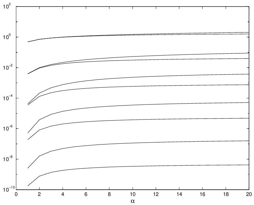
Since the eigenvalues of $Q$ come in reciprocal pairs, we only show the eigenvalues larger than 1; furthermore, we subtract 1 from them and show the result on a logarithmic scale (in order to clearly distinguish all eigenvalues). In the case depicted, $n=20$ , we see that 10 eigenvalues are larger than 1, for any value of the coupling constant $\alpha$ . Furthermore, the 10 remaining eigenvalues are all smaller than 1. This means that, in fact, $1$ is not included in the spectrum of $Q$ , which is completely at variance with the result for $Q^{\prime}$ of the purported reduced chain. Hence, we arrive at the statement that not even a single oscillator can be exactly decoupled from all the others by the application on an appropriate local symplectic transformation.

This analysis shows that the coupled bisected chain with nearest-neighbor interaction can not be reduced to a problem of only two pairs of interacting oscillators. In Section VII – equipped with further results from numerical investigations – we will discuss these findings and present an intuitive picture of the correlations present in the ground state of this system of coupled oscillators.

VI General bisections

In this section we turn towards more general problems, exhibiting less symmetry. As these problems are much more difficult to solve analytically, we basically have restricted ourselves to numerical calculations and we only give analytical results for small subproblems, valid in some asymptotic regime only.

VI.1 Asymmetrical bisections

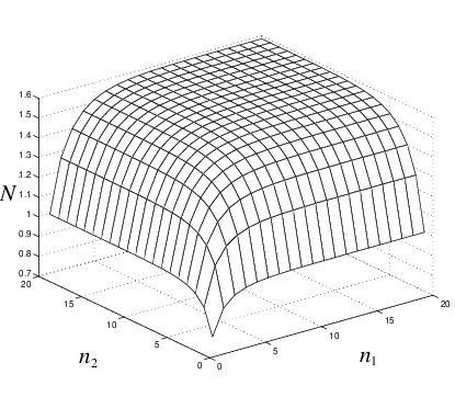
In Figures 4 and 5 we show the results of a numerical calculation for asymmetrically bisected chains with nearest-neighbor coupling.

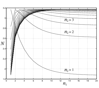
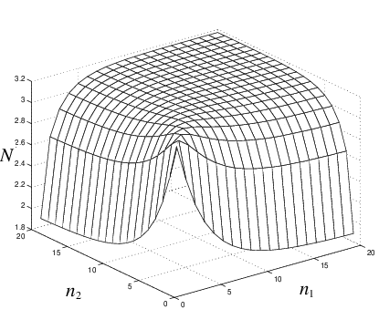
That is, the groups of oscillators have sizes $n_{1}\neq n_{2}$ . From these figures a number of features are immediately obvious. The most striking feature is the “plateau” in the entanglement that is reached whenever both groups are sizeable enough (say $n_{1},n_{2}>10$ , at least in the presented case for coupling strength $\alpha=20$ ). Of course, when $n_{1}=n_{2}$ , being the “diagonal” of the plot, we recover the result of Section IV that the log-negativity is independent of $n=n_{1}+n_{2}$ . From these figures we are led to conjecture that, in the case of nearest-neighbor coupling, the value of log-negativity for $n_{1}=n_{2}$ is an upper bound on the values for $n_{1}\neq n_{2}$ (not to be confounded with the result of Theorem 1, which says that this value is a lower bound for all symmetric bisections with general circulant couplings). Moreover, for general circulant couplings, we conjecture that an upper bound on $N(n_{1},n_{2})$ is given by $\lim_{m\rightarrow\infty}N(m,m).$ Another feature is that when, say, $n_{1}$ is kept fixed the log-negativity decreases with $n_{2}$ from a given value of $n_{2}$ onwards. This phenomenon is seen most clearly with small $n_{1}$ , particularly for $n_{1}=1$ . We will endeavour an intuitive explanation of these features below. In conclusion, we conjecture that, again for general circulant couplings, $\lim_{n_{2}\rightarrow\infty}N(1,n_{2})$ is a lower bound on $N(n_{1},n_{2})$ .

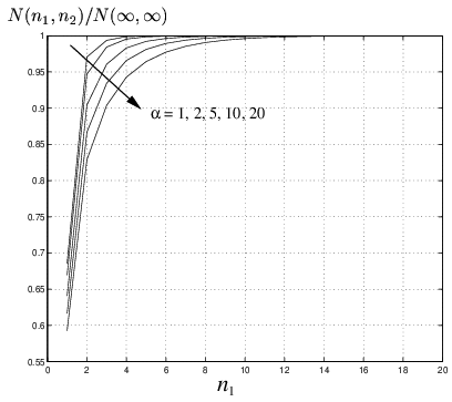
From Figure 6 we can see that the convergence of $N$ towards its plateau value $N(\infty,\infty)$ depends on the strength of the coupling $\alpha$ . For higher values, convergence is slower. What cannot be seen from this figure is that the actual plateau value is larger as well.

VI.2 Entanglement versus energy

It is interesting to compare the entanglement present in the chain ground state with its energy. We consider nearest-neighbor interaction only. We have shown in Section II that the ground state energy equals $(\hbar\omega/2){\mathrm{T}r}[V^{1/2}]$ . For zero coupling ( $V=\openone_{n}$ ) this gives just $n$ times the single-oscillator ground state energy $E_{0}=\hbar\omega/2$ , as expected. For large couplings $\alpha$ , we show that the ground state energy is of the order of $\sqrt{\alpha}nE_{0}$ .

From the proof of Theorem 2, we have that the eigenvalues $\lambda_{k}$ of $V$ are given by

\displaystyle\lambda_{k}=v_{0}+2v_{1}\cos(k2\pi/n)+2v_{2}\cos(2k2\pi/n)+\ldots.

The energy in terms of these eigenvalues is $\sum_{k=0}^{n-1}\lambda_{k}^{1/2}$ . For large values of $n$ , we can replace the discrete sum over $k$ by an integral in $x=2\pi k/n$ . For nearest-neighbor coupling, this yields:

$\displaystyle E$	$\displaystyle\approx$	$\displaystyle E_{0}(n/\pi)\int_{0}^{\pi}dx(v_{0}+2v_{1}\cos 2x)^{1/2}$
	$\displaystyle=$	$\displaystyle 2E_{0}(n/\pi)\int_{0}^{\pi/2}dx((v_{0}+2v_{1})-4v_{1}\sin^{2}x)^{1/2}$
	$\displaystyle=$	$\displaystyle 2E_{0}(n/\pi)\int_{0}^{\pi/2}dx(1+4\alpha\sin^{2}x)^{1/2}$
	$\displaystyle=$	$\displaystyle 2E_{0}(n/\pi)\sqrt{\alpha}\int_{0}^{\pi/2}dx(4\sin^{2}(x)+1/\alpha)^{1/2}.$

In the limit of $\alpha$ tending to infinity, the latter integral tends to $2\int_{0}^{\pi/2}dx\sin(x)=2$ , so that indeed

E\approx nE_{0}\frac{4}{\pi}\sqrt{\alpha}.

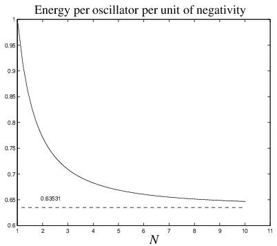
Recalling the exact formula for the log-negativity in the symmetrically bisected case, we have that the negativity (not the logarithmic one) is $\sqrt{1+4\alpha}$ . We thus find that the negativity is approximately proportional to the mean energy per oscillator. The exact values, calculated numerically, have been plotted in Figure 7. For $\alpha=0$ , the curve obviously goes through the point with mean energy equal to $E_{0}$ and negativity equal to 1. For $\alpha$ going to infinity, the mean energy goes to $(2/\pi)E_{0}=0.63662E_{0}$ times the negativity.

VI.3 Non-contiguous groups

From the above, one would get the impression that the mean energy gives a general upper bound on the amount of entanglement in the system (apart from a numerical factor). This is certainly not the case, because, until now, we only have investigated the cases where the two groups of oscillators were contiguous. In the following paragraph we look into the entanglement between non-contiguous groups. Specifically, we look at the extreme case of entanglement between the group of even oscillators and the group of odd ones. As can be seen from Figure 8, numerical calculations already show that the log-negativity tends to a constant times $n$ , the chain length. Therefore, in this case, the log-negativity can grow indefinitely large even when the mean energy is kept fixed. In view of this, it would be more correct to say that there are two contributions to the entanglement: one is the mean energy, which is directly related to the coupling strengths, and the second is the surface area of the boundary between the two groups of oscillators, which in the 1-dimensional case is just the number of points where the two groups “touch” each other. We will return to this issue in Section VII.

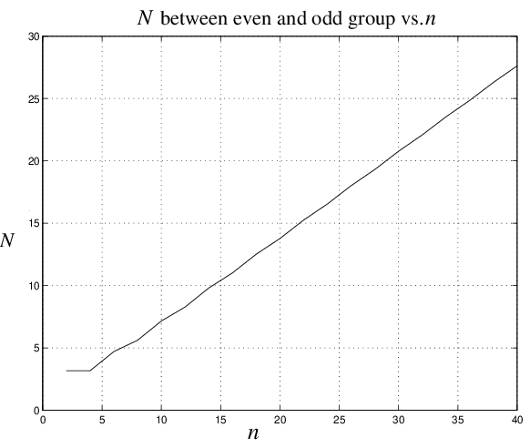
The validity of the purported linear relationship can be shown analytically in a rather simple way, yielding as a by-product an expression for the proportionality constant. First of all, the diagonal elements of the $P$ matrix for this configuration are 1 for odd index values, and -1 for even index values. The Fourier transform of $P$ , that is: $\Omega P\Omega^{\dagger}$ (see proof of Theorem 2), is equal to

\left(\begin{array}[]{cc}0&\openone_{n/2}\\ \openone_{n/2}&0\end{array}\right),

as is easily checked. We already have calculated the Fourier transform of the $V$ matrix, which again can be inferred from the proof of Theorem 2. It is given by $\Lambda=\Omega V\Omega^{\dagger}$ ; here, $\Lambda$ is a diagonal matrix with diagonal elements $\Lambda_{k}=v_{0}+2v_{1}\cos(2k\pi/n)+2v_{2}\cos(4k\pi/n)+\cdots$ , $0\leq k\leq n-1$ . Inserting this in the expression for the $Q$ -matrix gives:

Q=\Omega^{\dagger}\Lambda^{-1/2}\left(\begin{array}[]{cc}0&\openone_{n/2}\\ \openone_{n/2}&0\end{array}\right)\Lambda^{1/2}\left(\begin{array}[]{cc}0&\openone_{n/2}\\ \openone_{n/2}&0\end{array}\right)\Omega.

If we write $\Lambda$ in $2\times 2$ block form as

\left(\begin{array}[]{cc}\Lambda^{\prime}&0\\ 0&\Lambda^{\prime\prime}\end{array}\right),

the spectrum of $Q$ is the union of the spectrum of ${\Lambda^{\prime}}^{-1/2}{\Lambda^{\prime\prime}}^{1/2}$ and of ${\Lambda^{\prime\prime}}^{-1/2}{\Lambda^{\prime}}^{1/2}$ . Worked-out, this gives the eigenvalues $(\Lambda_{k+n/2}/\Lambda_{k})^{1/2}$ and $(\Lambda_{k}/\Lambda_{k+n/2})^{1/2}$ , for $0\leq k\leq n/2-1$ . Using the inherent symmetry that $\Lambda_{n-k}=\Lambda_{k}$ , the eigenvalues of $Q$ are

\left(\frac{\Lambda_{k}}{\Lambda_{n/2-k}}\right)^{\pm 1/2}.

The formula for the log-negativity obtained in Section III can be reformulated as minus the sum of the negative eigenvalues of $\log_{2}Q$ . In the present case we get as log-negativity

N=\frac{1}{2}\sum_{k=0}^{n/2}|\log_{2}\frac{\Lambda_{k}}{\Lambda_{n/2-k}}|.

For the nearest-neighbor Hamiltonian, this simplifies to

	$\displaystyle N$	$\displaystyle=$	$\displaystyle\frac{1}{2}\sum_{k=0}^{n/2}\|\log_{2}\frac{v_{0}+2v_{1}\cos(2\pi k/n)}{v_{0}-2v_{1}\cos(2\pi k/n)}\|$
		$\displaystyle=$	$\displaystyle\sum_{k=0}^{n/4}\log_{2}\frac{1+2\alpha(1+\cos(2\pi k/n))}{1+2\alpha(1-\cos(2\pi k/n))}$

for $n$ that are multiples of 4. For large $n$ , we can replace the discrete sum by an integral,

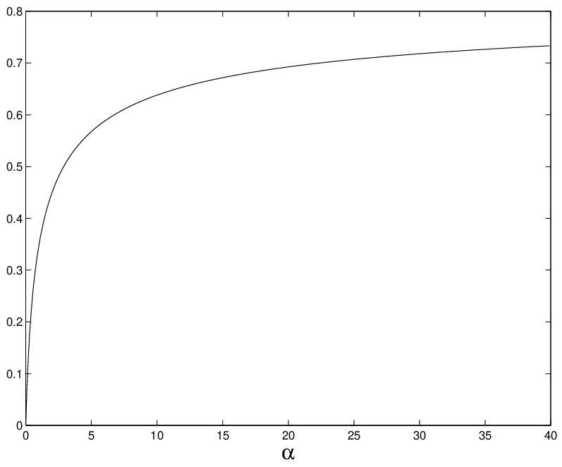
N\approx\frac{n}{2\pi}\int_{0}^{\pi/2}dx\log_{2}\frac{1+2\alpha(1+\cos(x))}{1+2\alpha(1-\cos(x))},

which indeed proves that, for large $n$ , the log-negativity is a linear function of $n$ . The integral itself cannot be brought in closed form. In Figure 9, we show the result of numerical calculations giving the asymptotic value of $N/n$ versus $\alpha$ .

VI.4 Effect of group separation

In the following paragraph, we give some results for contiguous groups that do not comprise the whole chain. In Figure 10 we consider a fixed chain of $n=40$ oscillators and look at the entanglement between two equally sized contiguous groups, in function of the group size and the separation between them. We define the separation as the number of oscillators in the smallest gap between the groups; since we are dealing with a ring, there are two gaps between the groups. Note that the log-negativity is plotted on a logarithmic scale. There are two main features in this figure. The first and least unexpected feature is that the entanglement decreases more or less exponentially with the separation. We believe that this is quite natural in view of the fact that the coupling between the groups also decreases with the distance.

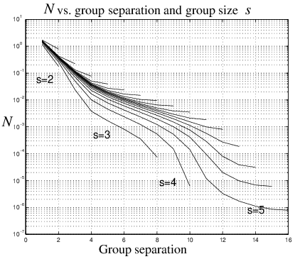
The more remarkable feature is that for small groups, the entanglement quickly becomes zero altogether, as measured by the logarithmic negativity. Bound entanglement Bound; Boundcv is of course not detected by this measure of entanglement, and it would be an interesting enterprise in its own right to study the structure of bound entanglement present in coupled oscillator systems. We will leave this, however, for future investigations. From now on, the term that no entanglement is present will be used synonymically with the statement that the logarithmic negativity vanishes.

For groups of size 1, the log-negativity is zero already at separation 1 (the gap consists of one oscillator). For groups of size 2, there is still entanglement at separation 1, but none at separation 2. The larger the groups, the larger the maximal separation for which there is still entanglement can be. One could try to interpret this by saying that there is a kind of threshold value below which entanglement drops to zero. However, this is more a reformulation of the results than an explanation, because it sheds no light on why this supposed threshold should depend on the group size.

To really explain what is happening, we need to take a closer look at the exact calculations. Consider first two groups of oscillators of size 2 and with separation 1; that is, group 1 is at positions 1 and 2, group 2 at 4 and 5. The $Q$ -matrix of this configuration (with $n=40$ and $\alpha=20$ ) has eigenvalues 2.063, 1.1339, 1.0938 and 0.88361. As one of the eigenvalues is smaller than 1, there is, indeed, entanglement present. We might be led to think that this entanglement is the cumulative result of the entanglement between the different oscillator pairs, (1,4), (1,5), (2,4) and (2,5), but this is not true, because these pairs are not entangled themselves: their separation is larger than 0. What is happening here is that the eigenvalues of the $Q$ -matrix belonging to pair (1,4), say, are 1.8065 and 1.1724, which are both larger than 1 and, therefore, do not count in the entanglement figure.

The resolution of this strange behaviour in terms of the separation is that the mere fact alone of having correlations between the groups (eigenvalues of $Q$ different from 1) is not enough to have entanglement. The correlations must be of special nature, namely: the eigenvalues of $Q$ must be smaller than 1. One could say that larger groups can more easily exhibit entanglement; their $Q$ matrix has a larger dimension and, hence, more eigenvalues, so that there are more opportunities for having at least one eigenvalue smaller than 1.

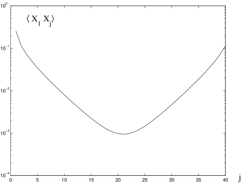
In this respect, it is interesting also to have a look at the classical correlations in the chain, i.e. the expectation values $\langle\hat{X}_{j}\hat{X}_{k}\rangle$ . From the treatment in Section II we immediately see that these correlations are given by the elements of the matrix $\gamma_{x}/2=V^{-1/2}/2$ . In the case of circulant symmetry, we only have to consider the first row of the matrix, giving the correlations between the first oscillator and any other one. Figure 11 shows these classical correlations for the system considered in Figure 10 ( $n=40$ , $\alpha=20$ ). As could be expected, these correlations decrease exponentially with the oscillator distance and, furthermore, never vanish completely.

VI.5 Thermal state

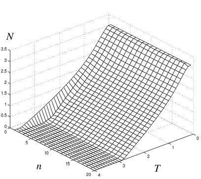
To conclude this section, we consider a thermal state instead of the ground state. The calculations are exactly the same in both cases, apart from the fact that in the covariance matrix there is an additional factor $\openone_{n}+2(\exp(\beta\sqrt{V})-\openone_{n})^{-1}$ to the $\gamma_{p}$ and $\gamma_{x}$ blocks ( $T=1/\beta$ ). The results are shown in Figure 12. One sees that for small temperatures the negativity is equal to the ground state negativity, and from some value onwards it starts to decrease more or less linearly with $T$ until there is no (free) entanglement at all anymore.

VII Discussion

The numerical results we have obtained in Section VI can be interpreted in a qualitative way, by means of two rules-of-thumb. These rules are not to be interpreted as strict mathematical statements; for that, we already have the exact formulas. The importance of the two rules is that they allow to reason about the dependence of entanglement on various factors, like group size, coupling strengths and group geometry.

The first rule is that, due to the coupling between the oscillators, the system exhibits inter-oscillator correlations which are decreasing with distance. This is a fairly natural statement, in view of the fact that the couplings between the oscillators are short-range as well. In a more mathematical way, one could consider the matrix $\gamma_{x}=V^{-1/2}$ , whose elements are the classical correlations $\langle\hat{X}_{j}\hat{X}_{k}\rangle$ . The $j$ -th row describes the correlations between the $j$ -th oscillator and all other oscillators. The correlations can thus, in a figurative way, be subdivided into packets, one packet for every row in the correlation matrix. For chains with a circulant potential matrix $V$ , it is self-evident that $\gamma_{x}$ is also circulant so that the correlation packets all have an identical shape (see Figure 13).

The second rule is that the entanglement between two groups of oscillators depends on the total amount of correlation between the groups. Again, this rule looks fairly innocuous and even trivial. However, combining the two rules readily shows why, in the case of contiguous groups, the entanglement in function of the group sizes should reach a plateau. Indeed, even while the total amount of correlation grows, more or less, linearly with the chain size, this has very little impact on the entanglement between the groups because it are only the correlation packets that straddle the group boundaries that enter in the bipartite entanglement figure. For large groups, most of the correlation packets describe correlations within the groups. What is important is the amount of correlations between the groups, and this quantity is virtually independent on the group size, provided the groups are so large they can accomodate most of the packets within their boundaries.

We must stress, however, that these two rules are of a qualitative nature. As noted already in Section VI, in the discussion of the dependence of entanglement on group separation, having correlations between the groups alone is not enough for having entanglement. The correlations must be such that the $Q$ matrix has at least one eigenvalue smaller than 1. The bottom line is in any case that one must go through the exact calculations to see whether or not there is entanglement.

Another effect that can be accounted for is the dependence of the log-negativity on the group size if at least one group is very small. If both groups are very small, say 1 oscillator both, then the packets are so wide they wind up along the chain and, therefore, cross every group more than once, adding to the entanglement figure a number of times. If one of the groups is kept fixed, and the other is made larger, the winding number of the packets decreases and so does the amount by which the packet is shared by the groups. This effect could explain the decrease of entanglement with growing $n_{2}$ . At this point, the qualitative reasoning again breaks down, however, since the reduction of the amount of sharing per packet is counteracted by an increase in the number of packets. To show that the balance is still in favour of an entanglement decrease, once again one really needs to go through the exact calculations; this is what we have done in Section IV. Nevertheless, the qualitative reasoning has the virtue that it shows what the main ingredients are. Furthermore, it immediately leads to the conjecture that the effect of decreasing entanglement would not occur in a chain that is not connected end-to-end, since no winding occurs there.

A numerical experiment immediately showed that this is exactly what happens, as witnessed by Figure 14.

One has to be careful, though, about how one “opens” the chain. To clearly show the disappearance of the winding effect, one has to make sure that opening the chain does not introduce side-effects. Particularly, the oscillators at both ends should still “see” the same springs as before opening the chain. One can take care of this by connecting the ends of the chain to two additional oscillators that are kept in a zero-energy state (i.e. with zero $X$ -variance; hence, they must be oscillators with infinite mass). At the level of the potential matrix, this means that the diagonal elements $V_{1,1}$ and $V_{n,n}$ are still $1+2\alpha$ , although the elements $V_{1,n}$ and $V_{n,1}$ are being set to zero. Noting the analogy between harmonic chains and transmission lines, we call this special connection process the termination of the harmonic chain. In transmission line theory, correct termination of a line (using appropriately matched impedances) is necessary to avoid signal reflections at the ends of the line. We believe that analogous reflection effects could be exhibited by non-terminated harmonic chains, but leave the investigation of this boundary phenomenon to future work.

Finally, for non-contiguous groups, and, specifically, for the entanglement between even and odd oscillators, the two rules-of-thumb correctly predict that the entanglement keeps increasing with growing chain length. Indeed, if $n$ grows, then the “boundary area” between the even and odd group also grows (linearly with $n$ ), in contrast with the contiguous groups, whose boundary area is fixed (1 for the open chain, 2 for the closed chain). Hence, the amount of correlations straddling the boundary should grow too. The exact calculation confirms this effect and shows a linear relationship between log-negativity and chain size. It would be interesting to investigate what happens in three-dimensional oscillator arrangements with couplings decreasing with distance. We believe that a similar relation will show up between entanglement between two groups and the area of the boundary between the groups. We leave this issue, however, for future investigations.

Acknowledgements.

This paper was benefited from very interesting conversations with C. Simon, R. Ratonandez, S. Scheel, M. Santos, and J. Harley. This work was supported by the European Union project EQUIP, the European Science Foundation programme on “Quantum Information Theory and Quantum Computing”, by a grant of the UK Engineering and Physical Sciences Research Council (EPSRC), and by a Feodor-Lynen grant of the Alexander von Humboldt Foundation.

References

(1) P. Horodecki and R. Horodecki, Quant. Inf. Comp. 1, 45 (2001); R.F. Werner, Quantum information – an introduction to basic theoretical concepts and experiments, in Springer Tracts in Modern Physics 173 (Springer, Heidelberg, 2001); W.K. Wootters, Quant. Inf. Comp. 1, 27 (2001); M.A. Nielsen and G. Vidal, Quant. Inf. Comp. 1, 76 (2001); M.B. Plenio and V. Vedral, Cont. Phys. 39, 431 (1998).
(2) N. Linden, S. Popescu, B. Schumacher, and M. Westmoreland, quant-ph/9912101; E.F. Galvao, M.B. Plenio and S. Virmani, J. Phys. A 48, 8809 (2000); S. Wu and Y. Zhang, Phys. Rev. A 63, 012308 (2001); A. Acin, G. Vidal, and J.I. Cirac, quant-ph/0202056.
(3) V. Vedral and M.B. Plenio, Phys. Rev. A 57, 1619 (1998); M.B. Plenio and V. Vedral, J. Phys. A 34, 6997 (2001); J. Eisert and H.J. Briegel, Phys. Rev. A 64, 022306 (2001).
(4) L. Vaidman, Phys. Rev. A 49, 1473 (1994); S. Braunstein, Nature 394, 47 (1998); N.J. Cerf, M. Levy, G. Van Assche, Phys. Rev. A 63, 052311 (2001); G. Lindblad, J. Phys. A 33, 5059 (2000); P. van Loock and S.L. Braunstein, Phys. Rev. A 63, 022106 (2001); T.C. Ralph, Phys. Rev. A 61, 022309 (2001); S. Parker, S. Bose, and M.B. Plenio, Phys. Rev. A 61, 032305 (2000); J. Eisert, C. Simon, and M.B. Plenio, J. Phys. A 35, 3911 (2002).
(5) Arvind, B. Dutta, N. Mukunda, and R. Simon, quant-ph/9509002; O. Krüger (Diploma thesis, TU Braunschweig, September 2001); R. Simon, Phys. Rev. Lett. 84, 2726 (2000); G. Giedke, L.-M. Duan, J.I. Cirac, and P. Zoller, Quant. Inf. Comp. 1, 79 (2001); J. Eisert and M.B. Plenio, Phys. Rev. Lett. 89, 097901 (2002); J. Eisert, S. Scheel, and M.B. Plenio, ibid. 89, 137904 (2002); J. Fiurášek, ibid. 89, 137904 (2002); G. Giedke and J.I. Cirac, Phys. Rev. A 66, 032316 (2002).
(6) R.F. Werner and M. Wolf, Phys. Rev. Lett. 86, 3658 (2001).
(7) M.A. Nielsen (PhD thesis, University of New Mexico, August 1998), also available at quant-ph/0011036.
(8) W.K. Wootters, quant-ph/0001114; K.A. Dennison and W.K. Wootters, quant-ph/0202048.
(9) K.M. O’Connor and W.K. Wootters, quant-ph/0009041; T.J. Osborne and M.A. Nielsen, quant-ph/0202162; H.J. Briegel and R. Raussendorf, Phys. Rev. Lett. 86, 910 (2001); P. Stelmachovic and V. Buzek, presented at Gdansk meeting 2001 (unpublished).
(10) C. Simon, Phys. Rev. A 66, 052323 (2002); J. Eisert and M.B. Plenio, Phys. Rev. Lett. 89, 137902(2002).
(11) K. Zyczkowski, P. Horodecki, A. Sanpera, and M. Lewenstein, Phys. Rev. A 58, 883 (1998); J. Eisert and M.B. Plenio, J. Mod. Opt. 46, 145 (1999).
(12) G. Vidal and R.F. Werner, Phys. Rev. A 65, 032314 (2002).
(13) J. Eisert (PhD thesis, University of Potsdam, February 2001).
(14) Horn and Johnson, Topics in Matrix Analysis (Cambridge University Press, Cambridge, 1991).
(15) J. Williamson, Amer. J. Math. 58, 141 (1936); R. Simon, E.C.G. Sudarshan, and N. Mukunda, Phys. Rev. A 36, 3868 (1987).
(16) R. Bhatia, Matrix Analysis (Springer, Heidelberg, 1997).
(17) M. Horodecki, P. Horodecki, and R. Horodecki, Phys. Rev. Lett. 80, 5239 (1998).