Focusing Vacuum Fluctuations II

In a previous paper FS00, henceforth I, we developed a geometric optics approach to the quantization of scalar and electromagnetic fields near the focus of a parabolic mirror. We found that there can be enhanced fluctuations near the focus in the sense that mean squared field quantities scale as an inverse power of the distance from the focus, rather than an inverse power of the distance from the mirror. These enhanced fluctuations were found to arise from an interference term between different reflected rays. In the present paper we extend the previous treatment. In I, only points on the symmetry axis were considered. Here we are able to treat points in an arbitrary direction from the focal line of a parabolic cylinder. We give more detailed numerical results which provide a fuller picture of the phenomenon of focusing of vacuum fluctuations. We also correct some erroneous results in Sect. V of I.

The outline of the present paper is as follows: In Sect. II, we review and extend some of the formalism used to calculate the mean squared scalar and electric fields, $\langle\varphi^{2}\rangle$ and $\langle{\bf E}^{2}\rangle$, near the focus. In Sect. III we derive some geometric expressions which are needed to study fluctuations at points off of the symmetry axis. In Sect. IV, the evaluation of integrals with singular integrands is revisited. Two different, but equivalent, approaches are discussed. A particular case where the integrals can be performed analytically is examined in Sect. V. More generally, it is necessary to calculate $\langle\varphi^{2}\rangle$ and $\langle{\bf E}^{2}\rangle$ numerically. A procedure for doing so is outlined in Sect. VI. Some detailed numerical results are also presented there. The limits of validity of our model and results will be examined in Sect. VII. This discussion will draw on some results on diffraction obtained in the Appendix. The experimental testability of our conclusions will be discussed in Sect. VIII. Finally, the results of the paper will be summarized in Sect. IX.

Units in which $\hbar=c=1$ will be used throughout this paper. Electromagnetic quantities will be in Lorentz-Heaviside units.

Here we will briefly review the geometric optics approach developed in I. The basic assumption is that we may use a ray tracing method to determine the functional form of the high frequency modes, which will in turn give the dominant contribution to the expectation values of squared field operators. We start with a basis of plane wave modes. The incident wave, for a scalar field, may be taken to be

with box normalization in a volume $V$. In the presence of a boundary, this is replaced by the sum of incident and reflected waves,

where the $f^{(i)}_{\bf k}$ are the various reflected waves. One could also in principle adopt a wavepacket basis, in which $F_{\bf k}$ is replaced by a localized wavepacket. Because the time evolution preserves the Klein-Gordon norm, if the various modes are orthonormal in the past, they will remain so after reflection from the mirror. Thus we can view Eq. (2) as the limit of a set of orthonormal wavepacket modes in which the modes become sharply peaked in frequency and hence delocalized.

It was shown in I that the renormalized expectation value of the squared scalar field is given by a sum of interference terms:

This renormalized expectation value is defined as a difference in the mean value of $\varphi^{2}$ with and without the mirror, and hence will vanish at large distances from the mirror. The various interference terms in the above expression yield contributions to $\langle\varphi^{2}\rangle$ which are proportional to the inverse square of the appropriate path difference. Thus in the vicinity of the focus, the interference terms between different reflected rays will dominate over that between the incident and a reflected ray. In the present paper, we will consider cases with no more than two reflected rays, and write

In the case of a parabolic cylinder, this may be expressed as

Here $\Delta\ell$ is the path difference for the two reflected rays, and the integration is over the reflection angle of one of the rays. The range is chosen so that each pair of reflected rays is counted once. The corresponding expression for the mean squared electric field near the focus of a parabolic cylinder is found in I to be

In this section, we wish to generalize some of the results of I concerning the incident and reflected rays in the presence of a parabolic mirror. Consider the geometry illustrated in Fig. 1. An incident ray at an angle of $\theta$ to the symmetry axis is reflected from the point $(x_{i},y_{i})$, and then reaches the point $P$ at an angle of $\theta^{\prime}$. We first need to find the relation between $\theta$ and $\theta^{\prime}$. Note that the reflected ray crosses the symmetry axis at a distance $c$ from the focus. It was shown in I that

However, from the law of sines, we have that

Hence we now have that

where

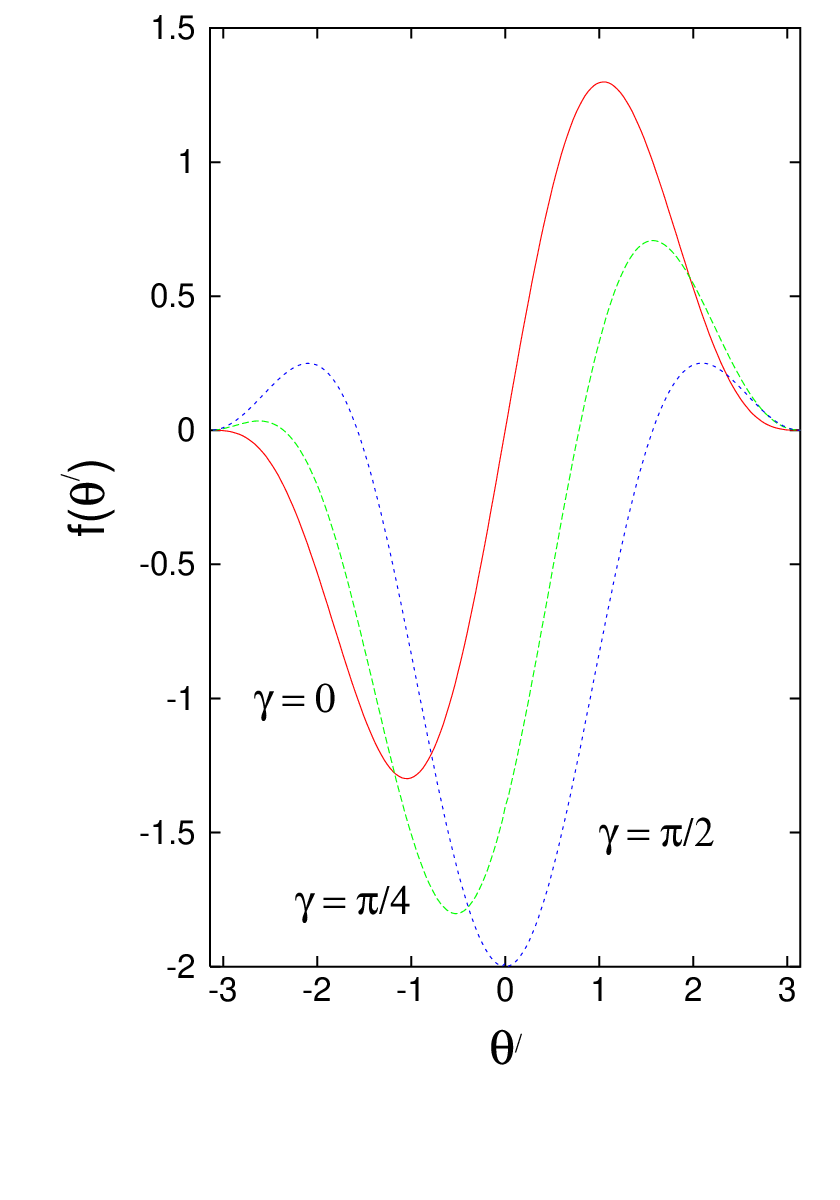
There will be multiply reflected rays whenever different values of $\theta^{\prime}$ are associated with the same value of $f$. The function $f(\theta^{\prime})$ is plotted in Fig. 2 for various values of $\gamma$. We can see from these plots that in general there can be up to four reflected angles $\theta^{\prime}$ for a given incident angle $\theta$. However, if the mirror size $\theta_{0}$ is restricted to be less than $2\pi/3$, then there will never be more than two values of $\theta^{\prime}$ for a given $\theta$. Throughout this paper, we will assume $\theta_{0}<2\pi/3$, and hence have at most two reflected rays for a given incident ray. The two reflected rays will occur at $\theta^{\prime}=\alpha$ and $\theta^{\prime}=\beta$, where

Our next task is to calculate the difference in path length, $\Delta\ell$, for these two reflected rays. Again, this is a generalization of a calculation given in I. Consider the situation illustrated in Fig. 3, where a reflected ray with angle $\theta^{\prime}$ reaches the point $P$ after reflecting from the point $(x_{i},y_{i})$ on the mirror. Let $s_{1}$ be the distance traveled after reflection, and $s_{2}$ be the distance traveled between when the ray crosses the line $x=x_{0}$ and when it reaches the mirror. Note that

Even if $x_{i}<0$, we can choose $x_{0}$ to be such that $s_{2}>0$. Next note that

The reflection point $(x_{i},y_{i})$ is the intersection of the line

with the parabola, given by

These relations lead to

We may now expand this expression to first order in $a/b$ and combine it with our previous expressions to show that, to first order,

Thus the magnitude of the path length difference for $\alpha$ and $\beta$, two different values of $\theta^{\prime}$, is

In the limit that $\gamma=0$, we obtain the result for $\Delta\ell$ used in I.

We can express Eq. (5) as

and Eq. (6) as

Here

and the integrations run over the full range for which there are two reflected rays, thus counting each pair twice.

The integrands of these integrals contain singularities within the range of integration. These singularities occur at a critical angle, $\theta_{c}$, at which $h$ vanishes linearly. Thus the $\langle\varphi^{2}\rangle$ integral contains a $(\alpha-\theta_{c})^{-2}$ singularity, and the $\langle{\bf E}^{2}\rangle$ contain a $(\alpha-\theta_{c})^{-4}$ singularity. These singularities are presumably artifacts of assuming perfect mirrors with sharp boundaries as will be discussed in Sect. VII. The singularity occurs when both $\alpha$ and $\beta$ are approaching $\theta_{c}$ from opposite directions. The critical angles $\theta_{c}$ are just the extrema of the function $f(\theta^{\prime})$.

Integrals with such singular integrands can be defined by a generalization of the principal value prescription. This generalization involves an integration by parts to recast the original integral as one containing a less singular integrand, plus surface terms. For example, we may use

to write

Similarly,

leads to

If $b>0$ and $a<0$, there were singularities in the original integrals which are replaced by integrable, logarithmic singularities. In all cases, the surface terms are evaluated away from the singularity and are hence finite. Note that we could have added additional polynomial terms on the righthand sides of both Eqs. (22) and (24). For example, we could replace $\ln x^{2}$ by $\ln x^{2}+c_{1}x+c_{0}$ in Eq. (22). However, the arbitrary constants $c_{0}$ and $c_{1}$ will cancel out between the two terms on the righthand side of Eq. (23) and hence can be ignored. A similar cancellation occurs if we add additional terms into Eq. (24).

If $f$ and a sufficient number of its derivatives vanish at the endpoints, then the surface terms vanish. In I, it was incorrectly argued that the surface terms which arise in the present problem can be ignored. It is true that if the reflectivity of the mirror falls smoothly to zero, the surface terms vanish. However, in this case it would be necessary to integrate explicitly the function which is falling smoothly to zero. If the reflectivity falls very rapidly at the edge of the mirror, its derivatives will be large, and effectively reproduce the surface terms. Thus, the explicit results given in Sect. 5 of I are incorrect. In Sects. V and VI of the present paper, we will give new results which replace and generalize the older results.

There is an alternative way to implement the above integration by parts prescription. This is simply to evaluate the integral as an indefinite integral, and evaluate the result at the endpoints, ignoring the singularity within the integration range. Even if it is not possible to find a closed form expression for the indefinite integral, one can expand the integrand in a Laurent series about $x=0$ and integrate term by term, using the relation

One can verify this relation for the case $a<0<b$ using the above integration by parts method.

The integrands in Eqs. (19) and (20) arise from the integrals

and

respectively. The integrals are understood to be performed with the aid of a convergence factor, such as ${\rm e}^{-\lambda\omega}$, with the limit $\lambda\rightarrow 0$ taken after integration. The singularities at $x=0$ are due to the contributions of arbitrarily large values of $\omega$. If there were to be a physical cutoff at high frequencies, then these singulariries would disappear. However, the integrals containing the singular integrands are independent of the cutoff in the limit that it occurs at sufficiently high frequencies. As an example, consider the function

As $\lambda\rightarrow 0$, $g_{2}(x,\lambda)\rightarrow-1/x^{2}$, but for $\lambda\not=0$, $g_{2}(x,\lambda)$ is finite for all $x$. Furthermore, if we integrate $g_{2}(x,\lambda)$ on $x$ through $x=0$, and then take the $\lambda\rightarrow 0$ limit, the result will be finite and the same as that obtained by the above formal procedures:

Similarly, if we define

then $g_{4}(x,\lambda)\rightarrow 6/x^{4}$ as $\lambda\rightarrow 0$. However,

Thus we can understand the physical meaning of the formal integration procedures discussed above as follows: they provide a shortcut method to obtain the results one would obtain by inserting a frequency cutoff in the $\omega$ integrals, and then removing this cutoff after integration over $x$.

One peculiar feature of our results will be that both $\langle\varphi^{2}\rangle$ and $\langle{\bf E}^{2}\rangle$ diverge for particular values of $\gamma$. This arises when $\theta_{c}$, the extremum of $f(\theta^{\prime})$, approaches the edge of the mirror, $\theta^{\prime}=\pm\theta_{0}$. The mathematical reason for the divergence is that one limit of integration is approaching a point at which $h=0$ and the integrand is singular. This corresponds to letting either $a\rightarrow 0$ with $b$ fixed, or $b\rightarrow 0$ with $a$ fixed, in Eq. (26). The physical origin of this singular behavior is that we have made two unrealistic assumptions. The mirror is assumed to be perfectly reflecting at all frequencies and to have sharp edges at $\theta^{\prime}=\pm\theta_{0}$. This will be discussed further in Sect. VII.

In general, the integrals for $\langle\varphi^{2}\rangle$ and $\langle{\bf E}^{2}\rangle$, Eqs. (5) and (6), respectively, can only be evaluated numerically. This is in part because the second reflection angle $\beta$ is implicitly given as a function of the first angle, $\alpha$. There is one case in which this relation may be written down in closed form. This is when $\gamma=\frac{\pi}{2}$, so the function $f(\theta^{\prime})$ is symmetrical about the origin. In this case, we have

and we can write

Similarly,

These expressions are plotted in Fig. 4. Note that both $\langle\varphi^{2}\rangle$ and $\langle{\bf E}^{2}\rangle$ can have either sign:

Both quantities seem to diverge in the limit that $\theta_{0}\rightarrow 0$

This divergence is a special case of the singularities arising when the edge of the mirror approaches an extremum of $f(\theta^{\prime})$.

We can go further and find the derivatives of both $\langle\varphi^{2}\rangle$ and $\langle{\bf E}^{2}\rangle$ with respect to $\gamma$, at $\gamma=\frac{\pi}{2}$. First, we need to find $\beta(\alpha)$ to first order in $\gamma-\frac{\pi}{2}$. We may expand the relation $f(\beta)=f(\alpha)$ to this order and show that

We can next expand $1/h^{2}$ and $1/h^{4}$ to first order in $\gamma-\frac{\pi}{2}$. The first order corrections are odd functions of $\alpha$ whose explicit forms we will not need.

The crucial effect of varying $\gamma$ slightly away from $\pi/2$ is to change the range of integration. First consider the case where $\gamma<\frac{\pi}{2}$. The integration range now becomes

where

To first order in $\gamma-\frac{\pi}{2}$, we can write

where the subscripts on $1/h^{2}$ denote the order in an expansion in powers of $\gamma-\frac{\pi}{2}$. The first term on the right hand side of Eq. (41) is just the zeroth order part given by Eq. (34). The next term vanishes because $(1/h^{2})_{1}$ is an odd function. The final term may be approximated using

This leads to

We may now repeat this procedure for $\gamma>\frac{\pi}{2}$. In this case, the range of integration is

and $\delta<0$, so the range of integration has again decreased. This causes the first order change in $\langle\varphi^{2}\rangle$ to have the same magnitude but the opposite sign from the previous case. Thus in all cases, we can write

A similar analysis may be applied to $\langle{\bf E}^{2}\rangle$ with the result

Thus both $\langle\varphi^{2}\rangle$ and $\langle{\bf E}^{2}\rangle$ have cusps at $\gamma=\frac{\pi}{2}$. The nonanalytic behavior is due to the fact that the range of integration decreases whenever $\gamma$ moves away from $\frac{\pi}{2}$ in either direction. As will be discussed in Sect. VII, the cusp is presumably an artifact of a sharp edge approximation, and should be smoothed out in a more exact treatment.

Apart from the special cases discussed in the previous section, it is necessary to evaluate $\langle\varphi^{2}\rangle$ and $\langle{\bf E}^{2}\rangle$ numerically. The first step is to find the second reflection angle $\beta$ as a function of the first reflection angle $\alpha$. This involves a straightforward numerical solution of the equation

Because we assume a restriction on the angle size of the mirror,

there will always be either one or no roots for $\beta$. Within the geometric optics approximation that we use, integrands are assumed to vanish in regions where there are no roots.

As was discussed in Sect. IV, there are at least two methods that may be used for explicit evaluation of the integrals which appear in the geometric optics expressions for $\langle\varphi^{2}\rangle$ and $\langle{\bf E}^{2}\rangle$. The first is an integration by parts, which replaces the singularity in Eqs. (19) and (20) by a logarithmic singularity. Here we will outline how this may be done explicitly. Consider first Eq. (19), which may be expressed as

Suppose that we are interested in integrating over the range $\alpha_{1}<\alpha<\alpha_{2}$ and that this range contains one point $\alpha=\alpha_{0}$ at which $h=0$. We can write

The quantity $(\alpha-\alpha_{0})^{2}/[h(\alpha,y(\alpha))]^{2}$ is finite at $\alpha=\alpha_{0}$. This expression may now be integrated by parts, as in Eq. (23). The derivatives of $h$ which arise are computed using Eq. (21) and the relation

An analogous procedure can be applied to $\langle{\bf E}^{2}\rangle$. The detailed expressions for $\langle\varphi^{2}\rangle$ and $\langle{\bf E}^{2}\rangle$ which result from this procedure are rather complicated, and will not written down explicitly.

The second method which may be employed is a variant of the direct integration illustrated in Eq. (26). The actual integrands in Eqs. (19) and (20) are too complex to integrate in closed form. However, we can use numerical integration of $1/h^{2}$ and $1/h^{4}$ in regions away from zeros of $h$ and direct integration of a series expansion in the neighborhood of a zero. The first step in the generation of the series expansion is to expand $\beta(\alpha)$ around $\alpha=\alpha_{0}$,

The coefficients are found by inserting this expansion into Eq. (47) and then expanding both sides of the resulting expression in powers of $\alpha-\alpha_{0}$. A few of the leading coefficients are

where the derivatives of $f$ are evaluated at $\alpha=\alpha_{0}$. The expansion for $y(\alpha)$ is then used to generate analogous expansions for $1/h^{2}$ and $1/h^{4}$, which are in turn integrated over the interval $\alpha_{0}-\xi_{0}<\alpha<\alpha_{0}+\xi_{0}$ using Eq. (26). The result is combined with the direct numerical integration outside of this interval. Here $\xi_{0}$ is an arbitrary small positive number. One of the tests of the numerical procedure is the independence of the results upon the choice of $\xi_{0}$.

We have developed numerical routines based upon both of the above procedures. The plots which are given below were created using a routine based upon the second method, with an expansion of $y$ to sixth order in $\alpha-\alpha_{0}$. The particular values of $\xi_{0}$ were in the range $0.1\leq\xi_{0}\leq 0.3$. In this range, the routine is relatively stable and insensitive to $\xi_{0}$. Smaller values of $\xi_{0}$ can lead to instability, as the contributions from $|x-x_{0}|>\xi_{0}$ and from $|x-x_{0}|<\xi_{0}$ are both large in magnitude and tending to cancel each other.

Numerical results for $\langle\varphi^{2}\rangle$ and $\langle{\bf E}^{2}\rangle$ for various values of $\theta_{0}$ are shown in Figs. 5-12 as functions of $\gamma$. In all cases, there are values of $\gamma$ at which $\langle\varphi^{2}\rangle$ or $\langle{\bf E}^{2}\rangle$ are singular in the model of a perfectly reflecting mirror with sharp edges. These points occur when an extremum of the function $f(\theta)$ sits at an edge of the mirror, $\theta^{\prime}=\pm\theta_{0}$. The values and slopes of $\langle\varphi^{2}\rangle$ and $\langle{\bf E}^{2}\rangle$ at $\gamma=\frac{\pi}{2}$ are in agreement with Eqs. (45) and (46). We can see from the graphs that for smaller mirrors, $\theta_{0}<\frac{\pi}{2}$, we have $\langle\varphi^{2}\rangle>0$ and $\langle{\bf E}^{2}\rangle<0$ everywhere. For larger mirrors, $\theta_{0}>\frac{\pi}{2}$, we have regions where $\langle\varphi^{2}\rangle>0$ and other regions where it is negative, and similarly for $\langle{\bf E}^{2}\rangle$. The signs of $\langle\varphi^{2}\rangle$ and of $\langle{\bf E}^{2}\rangle$ always seem to be opposite. The regions near $\gamma=\frac{\pi}{2}$ for larger mirrors where $\langle{\bf E}^{2}\rangle>0$ are of special interest. These are regions where an atom will feel an attractive force toward the focus, and thus has the possibility of being trapped.

In this section, we will discuss the likely ranges of validity of the model we have used to calculate $\langle\varphi^{2}\rangle$ and $\langle{\bf E}^{2}\rangle$. In particular, we have assumed a geometric optics approximation, and a mirror which is both perfectly reflecting and has sharp edges. Each of these assumptions will be examined critically.

In I, several possible experimental tests of the enhanced vacuum fluctuation near the focus were discussed. Here these tests will be reviewed and further discussed. The most direct test would seem to be to measure the force on an atom or other polarizable particle. In a regime where the atom can be described by a static polarizability $\alpha$, the force is ${\bf F}=-{\bf\nabla}V$, where

In the vicinity of the focus, we have found that

where $\Lambda$ is a dimensionless constant. For an atom in its ground state, Eq. (62) should be a good approximation when $a$ is larger than the wavelength associated with the transition to the first excited state.

One might try to measure the defection of atoms moving parallel to the focal line of a parabolic cylinder. The analogous experiment for a flat plate was performed by Sukenik et al Sukenik and confirmed Casimir and Polder’s theoretical prediction CP. In the present case, the expected angular deflection is

Here $m_{Na}=3.8\times 10^{-23}{\rm gm}$ and $\alpha_{Na}=3.0\times 10^{-22}{\rm cm}^{3}$ denote the mass and polarizability of the sodium atom, respectively. (Note that polarizability in the Lorentz-Heaviside which we use is $4\pi$ times that in Gaussian units.) If $t$ is of order $10^{-3}s$ (the time needed for an atom with a kinetic energy of order 300K to travel a few centimeters), and $z$ is of order $1\mu{\rm m}$, the fractional deflection is significant.

An alternative to measuring the deflection of the beam might be to measure the relative phase shift in an atom interferometer, which are sensitive to phase shifts of the order of $10^{-4}$ radians WPW. If one path of the interferometer were to be parallel to the focal line at a mean distance of $a$ and the other path far away, the phase difference will be

Both deflection and phase shift measurements would require the atoms to be rather well collimated and localized near the focal line.

Perhaps the most dramatic confirmation of enhanced vacuum fluctuations would be the trapping of atoms near the focus. This would require a mirror with $\theta_{0}>\frac{\pi}{2}$ so that there is a region with $\langle{\bf E}^{2}\rangle>0$. It would also require the atoms to be cooled below a temperature of about

Thus at temperatures of the order of $10^{-9}K$, atoms could become trapped in a region of the order of $1\mu{\rm m}$ from the focus. This type of trapping would be quite different from that currently employed Phillips in that it would require no applied classical electromagnetic fields.

The peculiar property that the force on an atom can be attractive from certain directions and repulsive from other directions requires some discussion. If one approaches from an attractive direction, the potential energy is becoming increasingly negative, $V\sim-1/a^{4}$, whereas from a repulsive direction it is becoming large and positive, $V\sim+1/a^{4}$. In both cases, $V\rightarrow 0$ for large $a$. At some minimum value of $a$, the inverse fourth power behavior has to be modified. Thus the exact potential energy $V(a,\gamma)$ must be a continuous function with a stable minimum, as illustrated in Fig. 13. Note that the requirement that $V\rightarrow 0$ for large $a$ in all directions rules out the possibility that there is only a saddle point, and no minimum. Although we can infer the existence of the minimum from our results, the detailed form of $V(a,\gamma)$ near the minimum could only be found by an analysis which goes beyond the approximations made in the present paper.

In this paper we have further developed a geometric optics approach to the study of vacuum fluctuations near the focus of parabolic mirrors. The main result of this approach is that the mean squared scalar field $\langle\varphi^{2}\rangle$ and mean squared electric field $\langle{\bf E}^{2}\rangle$ grow as inverse powers of $a$, the distance from the focus, for small $a$. The key justification of geometric optics is its self-consistency. When $\langle\varphi^{2}\rangle$ and $\langle{\bf E}^{2}\rangle$ are large, the dominant contributions must come from short wavelengths for which geometric optics is a good approximation. This was discussed more quantitatively in Sect. VII.

We have given some explicit analytic and numerical results for $\langle\varphi^{2}\rangle$ and $\langle{\bf E}^{2}\rangle$ near the focal line of a parabolic cylindrical mirror. In this paper, we restricted our attention to the case that the angular size of the mirror, $2\theta_{0}$, is less than $\frac{4\pi}{3}$. This insures that there are never more than two reflected rays for a given incident ray and simplifies the analysis We find that for smaller mirrors, $\theta_{0}<\frac{\pi}{2}$, $\langle\varphi^{2}\rangle>0$ and $\langle{\bf E}^{2}\rangle<0$ everywhere. In this case, an atom will feel a repulsive force away from the focus. For larger mirrors, $\frac{\pi}{2}<\theta_{0}<\frac{2\pi}{3}$, these mean squared quantities can have either sign, depending upon the direction from the focus. In directions nearly perpendicular to the symmetry axis, $\gamma\approx\frac{\pi}{2}$, we find $\langle\varphi^{2}\rangle<0$ and $\langle{\bf E}^{2}\rangle>0$. In this case, the force on an atom is attractive toward the focus and trapping becomes a possibility.

In the geometric optics approximation, the mean squared electric and magnetic fields are equal, so the local energy density is equal to $\langle{\bf E}^{2}\rangle$. Thus, when $\langle{\bf E}^{2}\rangle<0$, the local energy density is negative, and one has columns of negative energy density running parallel to the focal line of the parabolic cylinder.

The feasibility of experiments to observe the effects on atoms near the focus was discussed in Sect. VIII. Although the effects are small, it seems plausible that they could be observed.

*

References

- (1) L.H. Ford and N.F. Svaiter, Phys. Rev. A 62, 062105 (2000), quant-ph/0003129.
- (2) V. Sopova and L.H. Ford, Phys. Rev. D 66 045026 (2002), quant-ph/0204125.
- (3) L.H. Ford and N.F. Svaiter, Phys. Rev. D 58, 065007 (1998), quant-ph/9804056.
- (4) C.I. Sukenik, M.G. Boshier, D. Cho. V. Sandoghar, and E.A. Hinds, Phys. Rev. Lett. 70, 560 (1993).
- (5) H.B.G. Casimir and D. Polder, Phys. Rev. 73, 360 (1948).
- (6) See, for example, C.E. Wineland, D.F. Pritchard, and D.J. Wineland, Rev. Mod. Phys. 71, S253 (1999), and references therein.
- (7) See, for example, W.D. Phillips, Rev. Mod. Phys. 70, 721 (1998), and references therein.