Quantum information processing in bosonic lattices

The central problem in quantum information processing (QIP) qip is the ability to control a quantum system in order to achieve some predefined purpose like quantum computation (QC). In general, a quantum information processor is realized by assembling a large number of copies of a given quantum system e.g., a qubit, and by making these copies interact in a controlled coherent fashion. A crucial issue of any proposal for a QIP implementation is its scalability i.e., the realizability, at least in principle, of the above structure for an arbitrary large size. An appropriate architecture to achieve this last goal is naturally provided by a lattice with sites hosting the processing quantum systems.

In this paper we shall describe a general scheme for performing quantum computation with interacting bosonic particles in a lattice. The system under study is very general and several existing QC proposals could fit into this framework. These include optical qubits milburn; simple_qc; cerf, Josephson junction qubits jj and optical lattice loaded with ultracold bosonic atoms e.g., Bose-Einstein condensates (BECs) bec_lattice; vp; bec_qubit. Without focusing on any of these particular implementations, we will develop a general framework for encoding qubits and for performing universal quantum gates on such encoded qubits. Despite their highly practical relevance, we will not discuss decoherence issues since they are strongly dependent on the specific physical implementation.

Let us start by casting the problem we are going to address in a more precise control-theoretic fashion. The single mode Fock space will be denoted by $h:=\mbox{span}\{|n\rangle\}_{n=0}^{\infty}$. The Hamiltonian acting on ${\cal H}_{\Lambda}:=h^{\otimes\,L}$ that we would like to analyze is given by:

$$H({\cal V})=\sum_{i,j\in\Lambda}(V^{(2)}_{ij}n_{i}\,n_{j}+V^{(1)}_{ij}c_{i}^{\dagger}c_{j}+\mbox{H.c.})$$

(1)

where: (i) $\Lambda$ is an index set (the lattice vertices) with $L$ elements; (ii) $c_{j},\,c_{j}^{\dagger}(j\in\Lambda)$ are bosonic creation and annihilation operators and $n_{i}:=c_{i}^{\dagger}c_{i}$ the corresponding occupation numbers; (iii) ${\cal V}:=\{V^{(2)}_{ij}\}\times\{V^{(1)}_{ij}\}\subset{\mathrm{I\!R}}\times{\rm\kern 2.40005pt\vrule width=0.39993pt,height=6.28612pt,depth=-0.3014pt\kern-3.00003ptC},$ is the set of quasi-classical ’control’ parameters. The Hamiltonian (1) represents a generalized Bose-Hubbard model BH, the terms weighted by the $V^{(2)}_{ij}$’s account for the non-linear two-body interactions whereas the $V^{(1)}_{ij}$’s are one-body terms describing the hopping of the bosonic particles among the lattice sites. The interplay of these two terms is known to give rise to a rich quantum phase-diagram with insulating and superfluid regions bec_lattice; bec_mott.

The ultimate goal is to find an $M$-qubit encoding $e:({\rm\kern 2.40005pt\vrule width=0.39993pt,height=6.28612pt,depth=-0.3014pt\kern-3.00003ptC}^{2})^{\otimes\,M}\mapsto{\cal H}_{\Lambda}$ such that control on the parameters $V_{ij}(t)$ in (1) would enact universal computational capabilities on the code. In this paper we will propose such an encoding which will enable us to perform universal quantum computation on a suitable sector of the Fock space associated with the bosonic lattice Fock. It is worthwhile to keep in mind that even though we will consider only the ”spatial” interpretation of the single-particle modes i.e., spatially localized wave-functions, they could even be momentum modes or modes associated to any other single-particle wavefunction.

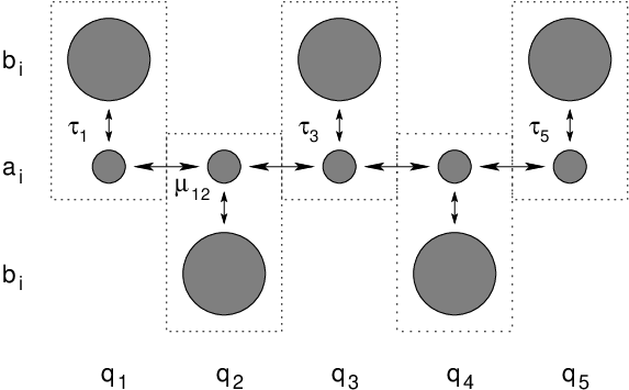We define the logical state of the qubit by the number of particles in the $a$ mode. Thus, $n_{a}=0$ defines the logical $|0\rangle_{\sf L}$ state and $n_{a}=1$ the logical $|1\rangle_{\sf L}$ state. The computational space is therefore restricted to $n_{a}\in\{0,1\}$ and we will show how to enforce this condition after each gate operation. It is important to stress that the subsystems which support our qubits are (finite-dimensional subspaces) of bosonic modes rather than particles. Therefore, the paradigm we adopt here concerning quantum entanglement for systems of indistinguishable particles is the one advocated in ref. fermi. We describe the main steps of any quantum computation scheme: universal set of gates, state preparation and measurement.

The following set of gates is universal for quantum computation gates: $\{\sf H,P_{\varphi},C_{\pi}\}$, where ${\sf H}=\frac{1}{\sqrt{2}}\pmatrix{1&1\cr 1&-1}$ is a Hadamard gate, ${\sf P}_{\varphi}=\mbox{diag}\,(1,\,e^{i\varphi})$ is a single-qubit phase shift, and $\sf C_{\pi}$ is a controlled sign flip. We use the more general controlled phase gate ${\sf C_{\varphi}}=\mbox{diag}\,(1,\,1,\,1,\,e^{i\varphi})$. We enact these gates by controlling the time dependence of the parameters characterizing the system. For the single-qubit gates we set all $\mu_{ij}=\chi_{ij}=0$ and we vary only the single-qubit parameters $\varepsilon_{\alpha,i}(t)$, $\gamma_{\alpha,i}(t)$ and $\tau_{i}(t)$ ($\alpha=1,2$). On the contrary, for the two-qubit gate, we keep constant the single-qubit parameters and we control only the inter-qubit tunneling rate $\mu_{ij}(t)$ or the Kerr coupling $\chi_{ij}(t)$.
Single-qubit gates. In the absence of any external coupling ($\mu_{ij}=\chi_{ij}=0$), the single-qubit Hamiltonian is (for simplicity we omit the qubit index $i$):

$$H_{1}=\varepsilon_{1}\,n_{a}^{2}+\varepsilon_{2}\,n_{b}^{2}+\gamma_{1}\,n_{a}+\gamma_{2}\,n_{b}+\tau(a^{\dagger}b+ab^{\dagger})$$

(4)

The total particle number $n=n_{a}+n_{b}$ is conserved, since $[H,n]=0$. Thus, the one-qubit Hilbert space splits into a direct sum ${\cal H}=\bigoplus_{n=0}^{\infty}{\cal H}_{n}$, as the Hamiltonian (4) leaves invariant the subspaces ${\cal H}_{n}$ with total particle number $n=\rm const$ and ${\rm dim}\,{\cal H}_{n}=n+1$. In view of this decomposition of the Hilbert space, we can relabel the Fock states as $|n_{a}\,n_{b}\rangle\equiv|n;\,n_{a}\rangle$. Thus, any vector can be written as $|\psi\rangle=\sum_{n}\sum_{i=0}^{n}c_{n,i}\,|n;\,i\rangle$. Since our initial state will be a Fock state and since the Hamiltonian conserves the total particle number $n$, the single-qubit wave-function at any time will always remain in the subspace ${\cal H}_{n}$, $|\psi(t)\rangle=\sum_{i=0}^{n}c_{n,i}(t)|n;\,i\rangle\in{\cal H}_{n}.$ Basically, the only degree of freedom left is the number of particles $i\,(=n_{a})$ in the $a$-mode.

For $\tau=0$, the Fock states $|n;i\rangle$ are are also energy eigenvectors, with eigenvalues given by (we omit the label $n$ since the total number of particle is conserved):

$$E_{i}\equiv\langle n;i|\,H\,|n;i\rangle=\varepsilon_{1}i^{2}+\varepsilon_{2}(n-i)^{2}+\gamma_{1}i+\gamma_{2}(n-i)$$

(5)

$i=0\ldots n.$ We also want our qubit states (defined as before $|0\rangle_{\sf L}\equiv|n;0\rangle$, $|1\rangle_{\sf L}\equiv|n;1\rangle$) to correspond to the degenerate ground state $E_{0}=E_{1}$. This implies the following energy degeneracy condition:

$$\varepsilon_{1}-(2n-1)\varepsilon_{2}+\gamma_{1}-\gamma_{2}=0$$

(6)

For the Hadamard gate, we keep $\varepsilon_{k}(t)$, $\gamma_{k}(t)$ constant (and satisfying the degeneracy condition (6)) and we allow only a time-dependent tunneling rate $\tau(t)$. Since the energy gap between the ground and the first excited state is $\Delta E\equiv E_{2}-E_{1}=4n\varepsilon_{2}+2(\gamma_{2}-\gamma_{1})=2(\varepsilon_{1}+\varepsilon_{2})$, we can treat the system in a first approximation as a degenerate two-level system, ignoring higher level transitions. The time evolution (up to a phase) is given by the operator $U(t)=e^{-i\sigma_{x}\int_{0}^{t}\tau(t^{\prime})dt^{\prime}}$, equivalent to a rotation around the $x$-axis ${\sf R_{x}}(\theta)\equiv e^{-i\theta\sigma_{x}}$. Then we can obtain the Hadamard gate as $\sf H=P_{\pi/2}\,R_{x}(\pi/4)\,P_{\pi/2}$. Similarly, we have ${\sf NOT}=i\,{\sf R_{x}(\pi/2)}$. In order to confirm this simple analysis, we have performed a full time-dependent simulation in the whole Hilbert space. We numerically integrate the Hamiltonian (4) for $n=30$. If we adiabatically switch the tunneling rate $\tau(t)$, we can control the population of higher levels (and hence the leakage form the computational space) to be negligible (in our simulation, this is less than $10^{-3}$ for a Gaussian pulse shape $\tau(t)$). The time scale required for performing single qubit gates is about one order of magnitude smaller than the one necessary for the two-qubit gate (see Fig. 2).

To enact the phase shift gate $\sf P_{\varphi}$ we keep the (intra-qubit) tunneling zero (therefore we always stay in the computational space) and we allow only a time dependence for (some of) the other parameters $\varepsilon_{k}(t)$, $\gamma_{k}(t)$, $k=1,2$. Since $\tau=0$, the time-dependent Hamiltonian is diagonal and we can solve the model analytically. Let $[0,\,T]$ be the time interval during which the gate acts. The time evolution of a Fock state is ($\hbar=1$): $|n;\,i\rangle\rightarrow e^{-iT\overline{E}_{i}}\,|n;\,i\rangle$, with $\overline{E}_{i}\equiv\frac{1}{T}\int_{0}^{T}E_{i}(t)dt$ the average value of $E_{i}(t)$ during the gate operation. Then the gate action on the basis states is:

$$U_{\varphi}=e^{-iT\overline{E}_{0}}\ \mbox{diag}\,(1,e^{-i\varphi})$$

(7)

with $\varphi=T(\overline{E}_{1}-\overline{E}_{0})$. In order to have $\varphi\neq 0$ we need to violate the energy degeneracy condition (6) by varying any of the four parameters $\varepsilon_{k}(t)$, $\gamma_{k}(t)$. From an experimental point of view, the self-interactions $\varepsilon_{k}$ might be harder to control, since they are related to the collision rates (in a BEC, for example). On the other hand, $\gamma_{k}$ are related to the energy offset of the trapping potential and are conceivably easier to control. Thus, we can keep constant any three of these parameters and control only the time variation of the remaining one (say $\gamma_{1}$). This method gives us considerable freedom in choosing the shape and duration of the pulses $\gamma_{1}(t)$ (the function $\gamma_{1}(t)$ is not even necessary to be continuous, it should be only integrable). Basically, the only condition is $\gamma_{1}(0)=\gamma_{1}(T)=\gamma_{2}-\varepsilon_{1}+(2n-1)\varepsilon_{2}$, such that the two-qubit states are again degenerate after the gate; this ensures that the phase difference between $|0\rangle_{\sf L}$ and $|1\rangle_{\sf L}$ is ’frozen’.

It is important to note that both rotation angles $\theta$ and $\varphi$ characterizing the single qubit gates depend only on the average values of $\tau(t)$ and $\gamma(t)$, respectively, and therefore they are relatively robust under small fluctuations of the control parameters (but they vary linearly with the gate time).

In the following we analyze in more detail a second universal (along with the one-qubit gates) Hamiltonian.
(ii) $H_{ij}=\varepsilon(n_{a,i}^{2}+n_{a,j}^{2})+\gamma(n_{a,i}+n_{a,j})+\mu_{ij}(a_{i}^{\dagger}\,a_{j}+a_{i}\,a_{j}^{\dagger})$. This is the Hamiltonian of two-qubits $i$ and $j$ interacting via the $a$-modes. It is identical to the one-qubit Hamiltonian (4), with $\varepsilon_{1,i}=\varepsilon_{1,j}=\varepsilon$ and $\gamma_{1,i}=\gamma_{1,j}=\gamma$, but now we also have $n_{a,i},n_{a,j}\in\{0,1\}$. Since the total number of particles is conserved $[H_{ij},n_{a,i}+n_{a,j}]=0$, we can neglect the constant term proportional to $\gamma$ and rewrite the Hamiltonian as (with the obvious notation $n_{i}\equiv n_{a,i}$, $n_{j}\equiv n_{a,j}$)

$$H_{ij}(t)=\varepsilon(n_{i}^{2}+n_{j}^{2})+\mu_{ij}(t)(a_{i}^{\dagger}\,a_{j}+a_{i}\,a_{j}^{\dagger})$$

(8)

Given the Hamiltonian (8), we want to find the control parameter $\mu_{ij}(t)$ such that the action of the gate is:

$$|n_{i}\,n_{j}\rangle\ {\rightarrow}\ e^{i\varphi_{n_{i}n_{j}}}|n_{i}\,n_{j}\rangle$$

(9)

This ensures that the total particle number for each qubit is conserved after the gate operation, i.e., there is no leakage from the computational space. Of course, during the gate operation this is not true, since intermediate states like $|02\rangle$ do not correspond to any logical state, but we will cancel these unwanted states dynamically. Again, let $[0,\,T]$ be the time interval during which the gate acts. There are three possible cases, depending on the initial state. Since the logical state $|n_{i}\,n_{j}\rangle_{\sf L}$ is the same as the Fock state $|n_{i}\,n_{j}\rangle$, we can omit the subscript ${\sf L}$ (keeping in mind that some intermediate states will not correspond to any logical state). The possible input states belong to different representations of $H_{ij}$ with total particle number $n=0,1,2$, respectively ($n\equiv n_{i}+n_{j}$).
(a) $|00\rangle$. This case is trivial, $|00\rangle\ {\rightarrow}\ |00\rangle$.
(b) $|01\rangle$ and $|10\rangle$. For $n=1$, we have $H_{ij}^{(1)}(t)=\varepsilon{\mathchoice{\rm 1\mskip-4.0mul}{\rm 1\mskip-4.0mul}{\rm 1\mskip-4.5mul}{\rm 1\mskip-5.0mul}}+\mu_{ij}(t)\sigma_{x}$ (the superscript (1) refers to the total particle number $n$). Since $[H_{ij}^{(1)}(t_{1}),H_{ij}^{(1)}(t_{2})]=0$ at all times, we can analytically integrate the time evolution to obtain:

$$U^{(1)}(T)=e^{-i\varepsilon T}({\mathchoice{\rm 1\mskip-4.0mul}{\rm 1\mskip-4.0mul}{\rm 1\mskip-4.5mul}{\rm 1\mskip-5.0mul}}\cos\omega_{1}T-i\sigma_{x}\sin\omega_{1}T)$$

(10)

with $\omega_{1}=\overline{\mu}_{ij}=\frac{1}{T}\int_{0}^{T}\mu_{ij}(t)dt$. Imposing condition (9), we require $\sin(\omega_{1}T)=0$. Therefore $\omega_{1}T=m_{1}\pi$, $m_{1}\in{\mathchoice{\hbox{$\sf\textstyle Z\kern-3.99994ptZ$}}{\hbox{$\sf\textstyle Z\kern-3.99994ptZ$}}{\hbox{$\sf\scriptstyle Z\kern-2.10002ptZ$}}{\hbox{$\sf\scriptscriptstyle Z\kern-0.99998ptZ$}}}$. This implies the following transformation for the basis states:

$$|01\rangle\ {\rightarrow}\ (-1)^{m_{1}}e^{-i\varepsilon T}|01\rangle$$

(11)

and similarly for $|10\rangle$.
(c) $|11\rangle$. For $n=2$, the Hamiltonian is:

$$H_{ij}^{(2)}(t)=\pmatrix{4\varepsilon&\sqrt{2}\mu_{ij}(t)&0\cr\sqrt{2}\mu_{ij}(t)&2\varepsilon&\sqrt{2}\mu_{ij}(t)\cr 0&\sqrt{2}\mu_{ij}(t)&4\varepsilon}$$

(12)

In general we cannot integrate this analytically. If $\mu_{ij}(t)=\rm const$, the exact time evolution is

	$\displaystyle|11\rangle\ {\rightarrow}\ e^{-3i\varepsilon t}\left\{|11\rangle\left(\cos\omega_{2}t+\frac{i\varepsilon}{\omega_{2}}\sin\omega_{2}t\right)-\right.$
	$\displaystyle\left.-\frac{i\mu_{ij}\sqrt{2}}{\omega_{2}}\sin\omega_{2}t\,(|02\rangle+|20\rangle)\right\}$		(13)

with $\omega_{2}=\sqrt{\varepsilon^{2}+4\mu_{ij}^{2}}$. Again, since we want to recover the $|11\rangle$ state after the gate operation, we impose the condition $\sin(\omega_{2}T)=0$, hence $\omega_{2}T=m_{2}\pi$, $m_{2}\in{\mathchoice{\hbox{$\sf\textstyle Z\kern-3.99994ptZ$}}{\hbox{$\sf\textstyle Z\kern-3.99994ptZ$}}{\hbox{$\sf\scriptstyle Z\kern-2.10002ptZ$}}{\hbox{$\sf\scriptscriptstyle Z\kern-0.99998ptZ$}}}$. In this case, the evolution of the state is $|11\rangle\ {\rightarrow}\ (-1)^{m_{2}}e^{-3i\varepsilon T}|11\rangle$. Together with the previous condition (i.e., $\omega_{1}T=m_{1}\pi$), we obtain

$$\frac{m_{2}}{m_{1}}=\frac{\omega_{2}}{\omega_{1}}=\sqrt{\frac{\varepsilon^{2}}{\mu_{ij}^{2}}+4}$$

(14)

Modulo single-qubit phases ${\sf P}_{\theta}^{\otimes 2}$, $\theta\equiv\pi(m_{1}-\sqrt{m_{2}^{2}-4m_{1}^{2}})$, the gate operation on the basis states $|n_{i}\,n_{j}\rangle$ is equivalent to

$$U(T)=\mbox{diag}(1,1,1,e^{i\phi_{11}})\equiv\sf C_{\phi_{11}}$$

(15)

with $\phi_{11}\equiv\pi(m_{2}-\sqrt{m_{2}^{2}-4m_{1}^{2}})$. In Fig. 2 we present a full time-dependent simulation for the evolution of the state $|11\rangle$ with $m_{1}=2$ and $m_{2}=6$. We choose a step function for the tunneling rate $\mu_{ij}(t)$. The simulation is in good agreement with the exact solution for constant tunneling presented above. After extracting the dynamical $e^{-i\varepsilon t}$ phase for each qubit, the $|11\rangle$ state picks up a phase $\phi_{11}/\pi=6-2\sqrt{5}\approx 1.53$, whereas the $|01\rangle$ and $|10\rangle$ states remain phaseless.

There is an important point to note here: the nonlinear term $\varepsilon(n_{i}^{2}+n_{j}^{2})$ in (8) is essential for enacting the gate. If $\varepsilon=0$ (or if we replace it with a linear one $\gamma_{i}\,n_{i}+\gamma_{j}\,n_{j}$), it can be shown that the gate would be equivalent to ${\mathchoice{\rm 1\mskip-4.0mul}{\rm 1\mskip-4.0mul}{\rm 1\mskip-4.5mul}{\rm 1\mskip-5.0mul}}$. This result is not surprising. The single-body operators entering our basic Hamiltonian (1) i.e., $\{c_{i}^{\dagger}c_{j}\}_{i,j=1}^{L}$ span, by commutation, a ${\cal A}_{L}\cong u(L)$ Lie algebra having $\hat{N}:=\sum_{i=1}^{L}c^{\dagger}_{i}c_{i}$ as central element. The lattice Fock space splits into $N+L-1\choose L-1$-dimensional invariant sectors of ${\cal A}_{L}$ labelled by the eigenvalues $N$ of $\hat{N}$ i.e., by the total number of bosons. In order to universally manipulate $M$ encoded qubits by using just the ${\cal A}_{L}$-elements one has to use $L\sim 2^{M}$ lattice sites. On the other hand our encoding scales linearly with the lattice size i.e., $M=L/2$. Thus, the nonlinear term in the Hamiltonian (1) provides an exponential reduction of resources.

The measurement technique is conceptually simple – we have to detect, for each qubit, the presence or the absence of one boson in the $a$-mode. For an optical lattice, this can be done by fluorescence: an atom present will fluoresce under the right laser illumination. The middle row of the qubit array will be a succession of dark (bright) spots, i.e., the atom is absent (present) in the $a$-mode, corresponding to qubit in state $|0\rangle_{\sf L}$ ($|1\rangle_{\sf L}$).

In conclusion, we have provided a further example of the paradigm of the so-called encoded-universality eu. A limited i.e., non-universal set of controllable interactions can still provide a full computational power in a suitable encoding subspace. We have presented a general framework for performing encoded universal QC on systems of self-interacting bosonic particles hopping on a lattice. Our strategy requires the ability to control in space and time the one-body couplings of the system. A summary of the parameter dependence for the gate operations is shown in Table 1 (only one of the two nonlinear interactions $\mu_{ij}$ and $\chi_{ij}$ are sufficient and therefore they can be used alternatively, depending on the system). Possible implementations of this scheme include optical qubits, Josephson junctions and BEC in optical lattices.

References

- (1) D.P. DiVincenzo and C. Bennett, Nature 404, 247 (2000).
- (2) G. J. Milburn, Phys. Rev. Lett. 62, 2124 (1989).
- (3) I. L. Chuang, and Y. Yamamoto, Phys. Rev. A52, 3489 (1995).
- (4) N. J. Cerf, C. Adami, and P. G. Kwiat, Phys. Rev. A57, 1477 (1998); quant-ph/9706022.
- (5) Y. Makhlin, G. Schön, and A. Shnirman, Rev. Mod. Phys. 73, 357 (2000).
- (6) D. Jaksch et al., Phys. Rev. Lett. 81, 3108 (1998).
- (7) R. Franzosi, V. Penna, and R. Zecchina, Int. J. Mod. Phys. B 14, 943 (2000); R. Franzosi, and V. Penna, Phys. Rev. A63, 043609 (2001).
- (8) Z.B. Chen, and Y.D. Zhang, Phys. Rev. A65, 022318 (2002).
- (9) M. P. A. Fisher et al., Phys. Rev. B40, 546 (1989).
- (10) M. Greiner et al., Nature 415, 39 (2002).
- (11) For massive particles the Fock space itself is not a physical state space (due to mass super-selection rules which forbid superpositions of vectors with different number of particles). In this case for any physical encoding must be included in a subspace with fixed particle number.
- (12) Bosons on ”lattices” with a complex structure have been studied e.g., R. Burioni et al, Europhys. Lett. 52, 251 (2000).
- (13) P. Zanardi, Phys. Rev. A65, 042101 (2002); P. Zanardi, X-G. Wang, Fermionic entanglement in itinerant systems, quant-ph/0201028.
- (14) A. Barenco et al., Phys. Rev. A52, 3457 (1995).
- (15) Excitonic creation operators , being fermionic bilinear, satisfy (hard-core condition). They are called pseudo bosons.
- (16) E. Biolatti et al., Phys. Rev. Lett. 85 5647 (2000); Phys. Rev. B65, 075306 (2002).
- (17) J. Kempe et al., Phys. Rev. A63, 042307 (2001); D. P. DiVincenzo et al, Nature 408, 339 (2000).