Dynamical Casimir Effect in a Leaky Cavity at Finite Temperature
Abstract
The phenomenon of particle creation within an almost resonantly
vibrating cavity with losses is investigated for the example
of a massless scalar field at finite temperature. A leaky cavity
is designed via the insertion of a dispersive mirror into a larger ideal
cavity (the reservoir).
In the case of parametric resonance the rotating wave approximation
allows for the construction of an effective Hamiltonian. The number
of produced particles is then calculated
using response theory as well as a non-perturbative approach. In
addition we study the associated master equation and briefly discuss
the effects of detuning.
The exponential growth of the particle numbers and the strong
enhancement at finite temperatures found earlier for ideal cavities
turn out to be essentially preserved.
The relevance of the results for experimental tests of quantum
radiation via the
dynamical Casimir effect is addressed. Furthermore the generalization
to the electromagnetic field is outlined.
PACS: 42.50.Lc, 03.70.+k, 11.10.Ef, 11.10.Wx.
I Introduction
Since the pioneering work of Casimir casimir the phenomena of quantum field theory under the influence of external conditions have attracted the interest of many authors, see e.g. bordag. The original prediction by Casimir, i.e., the attractive force generated between two perfectly conducting objects placed in the vacuum, has been verified in different experimental setups with relatively high precision lamoreauxmohideenbressi. However, its dynamic counterpart with non-stationary boundary conditions inducing interesting effects like the creation of particles out of the vacuum has not yet been observed rigorously in a corresponding experiment. The observation of quantum radiation could provide a substantial test of the foundations of quantum field theory and thus be of special relevance. Generally we understand the term quantum radiation to denote the conversion of virtual quantum fluctuations into real particles due to external disturbances. For the special case of the external disturbances being moving mirrors this phenomenon is known as the Dynamical Casimir effect.
These striking effects have been investigated by several authors, for an overview see e.g. bordag; jaekelreynaud and references therein. We will focus on the effect of particle creation within a constructed – resonantly vibrating – leaky cavity. This case is of special importance for an experimental verification of the dynamical Casimir effect since the generation of particles is enhanced drastically by resonance effects. Employing different methods and approaches it has already been shown for ideal cavities (see e.g. finitetemp) that under resonance conditions (i.e., when one of the boundaries performs harmonic oscillations at twice the frequency of one of the eigenmodes of the cavity) the phenomenon of parametric resonance (see e.g. jijungparksoh) will occur. In the case of an ideal cavity (i.e., one with perfectly reflecting mirrors) this is known to lead to an exponential growth of the resonance mode particle occupation numbers, cf. finitetemp; dalvit; dodonov1; dodonov2; dodonov3.
In view of this prediction an experimental observation of quantum radiation using the dynamical Casimir effect appears to be rather simple – provided the cavity is vibrating at resonance for a sufficiently long period of time. However, this point of view is too naive since neither ideal cavities do exist nor is it possible to match the external frequency to the fundamental eigenfrequency of the cavity with arbitrary precision. Consequently, it is essential to include effects of leaks as well as effects of detuning, see also golestanian.
Investigations concerning effects of losses have been performed for example in jrrad in 1+1 space-time dimensions based on conformal mapping methods as developed in davies. However, these considerations are a priori restricted to 1+1 dimensions and can not be obviously generalized to higher dimensions. In 3+1 dimensions the character of the mechanism generating quantum radiation – e.g., the resonance conditions – differs drastically from the 1+1 dimensional situation.
More realistic (3+1 dimensional) cavities were considered in leakydodonov where the effects of losses were taken into account by virtue of a master equation ansatz. However, this master equation had not been derived starting from first principles. It has already been noted in leakydodonov that the employed ansatz is adequate for a stationary cavity – but not necessarily for a dynamic one. In addition, most papers did not include temperature effects – which may contribute significantly in an experiment. It has been shown in Ref. finitetemp that for an ideal cavity the effect of particle production at finite temperature is enhanced by several orders of magnitude in comparison with the pure vacuum contribution.
In this article we will adopt the canonical approach which has proven to be general, successful, and is – in addition – also capable of including temperature effects. However, the aforementioned approach still lacks a generalization for systems with losses. We are aiming at providing a remedy in this field schaller.
This paper is organized as follows: In Sec. II we present a model system and derive the effective Hamiltonian for the resonance case. In Sec. III we will calculate the number of created particles in the cavity after one of the walls has performed resonant oscillations by means of response theory. In Sec. IV we will derive and solve the associated master equation and show consistency with the results obtained in Sec. III. In Sec. V a non-perturbative approach is presented and compared with the other results. We derive a treshold condition - valid for leaky cavities - for a possible detuning from the fundamental resonance in Sec. VI . We shall close with a summary, a discussion, a conclusion and an outlook.
Throughout this paper natural units given by will be used.
II General Formalism
II.1 The Leaky Cavity
We want to investigate the effects of a non-ideal cavity in view of the dynamical Casimir effect. For that purpose we have to construct a suitable model system. One simple way to do that is to insert a dispersive mirror into an ideal cavity while keeping all other walls perfectly reflecting. Thereby two leaky cavities are formed. Particles in the left imperfect cavity are now able to leave into the right larger box (the reservoir). For reasons of simplicity we consider a rectangular cavity as depicted in Fig. 1.

The setup in Fig. 1 is not a new idea. A similar – but static – system has already been treated in scully; banachloche. However, here in addition the left wall is moving with a prescribed trajectory during the time interval . For ideal cavities this is known to lead to a squeezing of the vacuum state which causes the creation of particles inside the cavity, see e.g. finitetemp.
Note that we are assuming a finite reservoir with a discrete spectrum instead of an infinite one leading to a continuum of modes. Since, in an experimental setup, the vibrating cavity will most likely be surrounded by walls, etc. (imposing additional boundary conditions), this assumption should be justified.
Assuming a surrounding perfectly reflecting wall is a first idealization of the real situation. However, in order to minimize the error obtained by this procedure the experiment could be designed in this way, see also Fig. 8 in section IX below.
The ideal mirrors can be simulated by infinitely high potential walls inducing Dirichlet boundary conditions. For the additional dispersive mirror we use the -type model potential proposed in Ref. calogeracos; salomone
see also Fig. 2. The parameter represents the transmittance of the internal mirror, whose reflection and transmission amplitudes are determined as calogeracos
| (4) |
Note that the general procedure presented in this article is independent of the particular form of the potential – the aforementioned one has just been chosen for convenience. For a more realistic scenario one could apply square-well or Gaussian potentials. In a realistic experiment where one would want to create photons instead of scalar particles a dispersive mirror could be realized using a thin dielectric slab with a very high dielectric constant. Such a mirror could then be approximated by a space-dependent permittivity . This will be addressed in Sec. X.2.

II.2 Hamiltonian
Throughout this article we will use the notation of tremblingcav where the particle production in an ideal vibrating cavity was calculated – for a more general treatment see e.g. blackhole. We consider a massless and neutral scalar field coupled to an external potential:
| (5) |
The perfect mirrors can be incorporated by imposing the corresponding boundary condition on . By expanding the field
| (6) |
into a complete and orthonormal set of functions satisfying
| (7) | |||
| (8) | |||
| (9) |
one can reach a more convenient form suitable for doing calculations. Since is a real field, we can choose the set to be real. Note that the time dependence of eigenfunctions and eigenfrequency is solely induced by the moving boundary. Inserting this expansion into Eq. (5) transforms the Lagrangian into tremblingcav
| (10) | |||||
where is an antisymmetric matrix given by
| (11) |
This matrix describes the coupling strength between two different modes. We introduce the canonical conjugated momenta
| (12) |
Furthermore we apply the usual Legendre transform to a Hamiltonian representation and perform the quantization. This yields
| (13) |
The above Hamiltonian can be sub-classified into
| (14) |
where the single Hamiltonians are given by
| (15) | |||||
| (16) | |||||
| (17) |
The deviation denotes the difference of the (squared) time-dependent eigenfrequencies from the unperturbed ones . The first term is the Hamiltonian of harmonic oscillators. The remaining terms will further on be called squeezing interaction Hamiltonian and velocity interaction Hamiltonian. We want to point out that in the case of a static system (where the eigenfunctions and eigenfrequencies are constant in time) the complete interaction Hamiltonian will vanish. The derivation of the eigenfunctions and will be treated in the following subsection.
II.3 Eigenmodes
As has already been mentioned, we want to find a set of functions satisfying . Any time dependence can only be induced by the moving boundaries. At first we will just consider the spatial dependence i.e., the stationary problem. The differential equation can be treated using the separation ansatz where depends only on the coordinate parallel to the wall velocity and is dependent on the perpendicular coordinates. For the special case of our model system this means leading to the trivial and dependence of the eigenfunctions
| (18) | |||||
| (19) |
with and denoting the dimensions of the cavity and the frequencies relating via
| (20) |
The remaining differential equation reads
| (21) |
where the Dirichlet boundary conditions coming from the perfect mirrors on either side can be satisfied by the ansatz
The eigenfunctions have to obey the continuity conditions calogeracos
| (26) | |||||
| (27) |
where the latter can be obtained via integration. These conditions can be combined to an eigenvalue equation for
| (28) |
Though there is no obvious analytical solution of this equation, a numerical solution can always be obtained for given cavity parameters . However, via introducing the dimensionless perturbation parameter it is also possible to obtain an approximate analytical solution. Note that this parameter is small in the limit of the internal mirror being nearly perfectly reflecting. Since the trigonometric functions are very sensitive to small frequency variations one can solve the equation using a series expansion in . It is obvious that if the right hand side goes to one of the addends or even both can become relevant. This depends on the ratio and its inverse which are both assumed to be non-integer numbers in the following non-perturbative calculations implying that only one of the addends is dominating. Accordingly, expanding around the poles of one addend one yields a polynomial that can be solved for as a series expansion in . Depending on the chosen addend one obtains two sets of approximate eigenfrequencies
| (29) | |||||
which constitute a determining polynomial for . Note that the index is a multi-index, where and stand for left-dominated and right-dominated, respectively. However, it can be shown easily that the quality of the linear (in ) approximation suffices already for moderate values of . The insertion of (II.3) into the ansatz (II.3) leads to two classes of eigenfunctions: left-dominated and right-dominated, respectively. The differences between those are clearly visible in Fig. 3.
In order to avoid the confusion arising from a set of perturbation parameters we will introduce the fundamental one via
| (30) |
to which all others are evidently related via . Note that this distinction between the classes of eigenfunctions is applicable only for small values of .
Consequently, the eigenfunctions can be labeled by multi-indices : 3 quantum numbers and a flag denoting the class (right- or left-dominated, respectively) of the eigenfunction.

Now we want to consider the effect of one moving boundary. It is taken into account by substituting everywhere in the eigenmodes and -frequencies. Thereby a time dependence of the eigenfunctions as well as of the eigenfrequencies is introduced. This induces a non-vanishing coupling matrix as well as the frequency deviation . For small oscillations of the boundary
| (31) |
with a small amplitude it will be useful to separate the time dependence using
| (32) | |||||
The geometry factor is approximately constant in this case. Consequently, one is lead to
| (33) |
Since the time-dependence of the right-dominated modes is less complicated than that of the left-dominated ones, it is advantageous to exploit the antisymmetry of which also implies an antisymmetry of . For the following calculations the coupling of the lowest left-dominated mode to some right-dominated one will be of special relevance. The and integrations simply generate Kronecker symbols and therefore the geometry factor results as
| (34) | |||||
II.4 Canonical Quantization
Aiming at the calculation of possible particle creation effects (expectation values of particle number operators) it is convenient to introduce the creation and annihilation operators
| (35) |
obeying the usual bosonic equal time commutation relations
| (36) |
These operators diagonalize the free Hamiltonian
| (37) |
The following calculations will most conveniently be done in the interaction picture where the dynamics of an observable is governed by
| (38) |
For reasons of generality and to include finite temperature effects we describe the state of a quantum system by a statistical operator whose dynamics is determined by the von Neumann equation
| (39) |
Note that this equation without any explicit time dependence leads to an unitary time evolution, see also finitetemp and Sec. IV.
In this picture the time dependence of the creation and annihilation operators turns out to be
| (40) |
However, this trivial time dependence gives rise to the possibility of parametric resonance which enhances the chances to verify the effect of particle creation experimentally. Further-on we will denote the initial creation and annihilation operators by . Note that in this picture the particle number operator is time independent for all modes.
II.5 Rotating Wave Approximation
In the interaction picture the time-evolution operator is given by
| (41) |
where denotes time-ordering. If the interaction Hamiltonian leads to small corrections, the usual procedure is to apply perturbation theory via expanding the exponential. Evidently, this would imply that is close to the identity. On the other hand, in order to make an experimental verification of quantum radiation feasible, the time-evolution operator should deviate significantly from the identity. Therefore a different approximation needs to be found. For the case of parametric resonance this may be accomplished via applying the rotating wave approximation (RWA), see e.g. finitetemp; law; wuchuleung. Within this scenario the left boundary performs harmonic oscillations obeying with the dimensionless amplitude11 1 For uniqueness we restrict ourselves to . and the external vibration frequency during the time interval . This also implies an oscillating time-dependence of the frequency deviation and coupling matrix
| (42) | |||||
| (43) |
see also Sec. II.3. Together with the trivial time-dependence of the ladder operators (40) in the interaction picture this enables us to perform the RWA. Expanding the time evolution operator (41) into an infinite series one can treat the time-ordering terms in the following way: In analogy to
| (44) | |||||
one can rewrite all these terms to yield a multiple product of Hamiltonians without time-ordering and terms involving commutators with Heaviside step functions. In the resonance case, i.e., when the terms with commutators can yield nothing but strongly oscillating integrands finitetemp, as can also be seen by Fourier-expanding the involved Hamiltonians. With the duration of the perturbation being sufficiently long, i.e., with , the contribution of these terms to (41) will be comparably small. As a consequence, time-ordering can be neglected to all orders within the RWA.
The remaining integrals – without time-ordering – factorize and can be resummated to yield an effective time evolution operator
| (45) |
where the effective interaction Hamiltonian
| (46) |
still has to be calculated. The above time integration involves many oscillating terms. Again, with the duration of the vibration being sufficiently long , i.e., after many oscillations, the time-integrated interaction Hamiltonian can be approximated in the following way: Since the time average of purely oscillating terms is rather small compared to that of constant contributions we may neglect the former ones. As a result, in the series expansion of the time-evolution operator only those terms where the oscillation of the ladder operators is compensated by the external vibrations – represented by and , respectively – will be kept. Strictly speaking, in the above equation terms of are neglected by the RWA if holds. The terms with – i.e., exactly the terms in which the oscillations of the creation and annihilation operators (40) are compensated by the external time dependence and ] – will be kept. (Note that terms with do not occur.)
The general squeezing interaction Hamiltonian reads
| (47) | |||||
Accordingly, within the RWA only the terms fulfilling the squeezing resonance condition, see also e.g. leakydodonov; finitetemp; quantumrad; braginsky
| (48) |
will be kept. In general can also be a right-dominated mode, but note that in this case the effective squeezing Hamiltonian would be of , since according to (II.3) the right-dominated eigenfrequencies do not depend on up to . Therefore we will restrict ourselves to left-dominated modes and among those in particular to the lowest one, i.e., as commonly done we consider the case of fundamental resonance
| (49) |
From now on this mode will be abbreviated by the index throughout this publication. Consequently, by virtue of
| (50) |
an effective squeezing Hamiltonian can be derived
| (51) |
where is given by
| (52) |
Obviously is a generator for a squeezing operator for the mode with being the squeezing parameter.
The same procedure can be applied for the velocity interaction Hamiltonian which reads in the vibration case
| (53) | |||||
However, the occurrence of inter-mode couplings now results in a different resonance condition (see also finitetemp; quantumrad)
| (54) |
Depending on the frequency spectrum of the cavity under consideration this resonance condition might be fulfilled by several pairs , but here we will assume for simplicity that only one such pair exists. Though in any case via
| (55) |
an effective velocity Hamiltonian can be derived, two major distinctions should be made.
coupling
. In this case one yields an effective velocity Hamiltonian given by
| (56) | |||||
which is a non-diagonal multi-mode squeezing Hamiltonian. Note that if one wants to fulfill squeezing and velocity resonance conditions simultaneously (), the number of possible combinations reduces significantly, since then the velocity resonance condition can not be fulfilled by two distinct left-dominated modes. For reasons of brevity we do not consider this case here.
coupling
. Here the resulting effective velocity Hamiltonian does not resemble a squeezing but a hopping operator
| (57) | |||||
This coupling is of special interest since if one does not insist on simultaneously fulfilling both resonance conditions – parametric resonance might perhaps still be induced by lower external frequencies whose generation would be simpler in an experiment, see also Sec. V.3. In the case of simultaneously fulfilling both conditions several combinations may arise.
- •
The frequencies both belong to either right- or left-dominated modes. In dalvit it has been shown that for an ideal cavity with special dimensions, e.g. a cubic one, a strong inter-mode coupling can occur. In that case a much smaller exponential particle creation rate has been found. Therefore in view of an experimental verification this case is counterproductive and not considered here. Instead we propose a cavity with transcendental ratios of the dimensions such that there is no resonant inter-mode coupling of similar-dominated modes. In any case such a coupling would certainly require large quantum numbers of the involved modes.
- •
The frequency represents a right-dominated mode and some left-dominated mode, respectively. The lowest possible right-dominated frequency would then be obtained when . As an example, this case will be considered here. We want to stress that the used methods are nevertheless applicable to any possible combination of couplings.
Note that the situation would be completely different in 1+1 space-time dimensions where – due to the equidistant spectrum – the velocity term always contributes, see e.g. finitetemp; dodonov1; dodonov2; dodonov3; dodonov4; dodonov5; dodonov6. The coupling right-dominated mode fulfilling will further-on be denoted with the index . Accordingly, in our considerations the velocity Hamiltonian reads
| (58) |
with
| (59) |
being the velocity parameter of the system. Since [see also (34)] it follows that in the limiting case of a nearly perfectly reflecting mirror22 2 Note that for inter-mode coupling between modes of the same region – the corresponding scenario has been assumed in dalvit for an ideal cavity where one only has one region – the velocity parameter would be of instead of .. This hopping operator is consistent with the visual picture of a semitransparent mirror.
II.6 Response Theory
We assume our system to be initially in a state of thermal equilibrium that can be described by the canonical ensemble
| (60) |
with denoting the initial inverse temperature. The expectation value of an explicitly time-independent operator at time is given by
| (61) | |||||
where denotes the anti-chronological operator (anti-time ordering) – for a more involved discussion see e.g. finitetemp.
If the interaction Hamiltonian represented a small correction, one could expand the time-evolution operator into a perturbation series yielding a series expansion for . However, for the resonance case this procedure is not justified: In the rotating wave approximation in Sec. II.5 the interaction Hamiltonian simplified to
| (62) |
which implies for the time-evolution operator
| (63) |
The whole expression for computing the expectation value of an operator now becomes much simpler
| (64) | |||||
but since the correction is not small in the case of interest above expression is still not practical for applying perturbation theory. Exploiting the smallness of the velocity Hamiltonian it will prove useful to separate the two Hamiltonians. This can be achieved with the ansatz
| (65) |
with being an auxiliary operator. Differentiation with respect to yields a differential equation that can be solved for using the initial condition . Introducing the parameter ordering in analogy to time ordering () the solution for can be cast into the form
| (66) |
Here the squeezed effective velocity Hamiltonian has been introduced
| (67) |
which is now dependent on the parameter . Further-on we shall denote squeezed operators by calligraphy letters. By inserting above equations into the expectation value (64) one yields
| (68) | |||||
Please note that in this representation also the observables are squeezed
| (69) |
but here using the physical perturbation time . We will refer to this picture as the squeezing interaction picture. Unfortunately the parameter ordering is reintroduced by this procedure but as the advantage of these manipulations we are now able to expand the expectation value into a perturbation series with powers of . Keeping only terms to second order one finds
| (70) | |||||
which is now a practical expression for calculating expectation values.
III The Quadratic Response
III.1 Squeezing
According to the results of Sec. II.6 in the squeezing interaction picture both particle number operator and the effective velocity Hamiltonian have to be squeezed. The squeezing operator
| (71) |
implies the following well-known transformation rules (see e.g. mandelwolf)
| (72) | |||||
| (73) | |||||
which can also be envisaged as a Bogoliubov transformation of the ladder operators. Due to the commutation relations (II.4) other modes than the fundamental resonance mode are not affected by squeezing. Inserting the above expressions into the effective velocity Hamiltonian (58) one can easily derive its squeezed counterpart
| (74) | |||||
Note that the squeezed effective velocity Hamiltonian is now dependent on the parameter and that it is still of which justifies a perturbation-like treatment.
The same can be done for the particle number operators where again only the fundamental resonance mode is affected
| (75) | |||||
For brevity we will denote the hyperbolic functions by
| (76) |
throughout this paper.
III.2 Expectation Values
Since we are mainly interested in the phenomenon of quantum radiation and thus therefore in the calculation of the cavity particle content after a time when the disturbance has ended. Due to the dynamical disturbance the system leaves the thermodynamic equilibrium, see also finitetemp. The quadratic response of the expectation value of the particle number operator can be calculated via substituting in equation (70). However, since the initial statistical operator involves arbitrarily high powers in , it is practical to rewrite the expression obtained from (70). Utilizing the invariance of the trace under cyclic permutation and the property of time ordering
| (77) | |||||
the expectation value of interest can be cast into the more convenient form
| (78) | |||||
This form is now suitable for evaluating the traces since all commutators only concern a finite number of creation or annihilation operators. Thus the quadratic response can be brought in relation with the initial particle contents of the cavity (Bose-Einstein distributions)
| (79) | |||||
| (80) |
where stands for the initial inverse temperature of the system. These mean occupation numbers incorporate the whole temperature dependence of the quantum radiation – as long as the back-reaction of the field on the moving mirror can be neglected. As we shall show later, the lowest order term () is in agreement with the results of an ideal cavity, as was considered for example in finitetemp; dalvit. Also, since contains only odd powers of creation and annihilation operators for a single mode, the linear response vanishes. Generally, every trace involving an odd power of ladder operators vanishes and as well as do only contain even powers. Hence the last trace in Eq. (78) constitutes the quadratic answer. In contrast to an ideal cavity the terms with time ordering are here especially important since they will be found to produce leading order terms.
III.3 Particle Creation
Using the squeezed operators (74) and (75) it is now straightforward to compute the commutators and the traces in the expectation value (78). As a result one finds for particles in the fundamental resonance mode
| (81) | |||||
As was anticipated, the lowest order term is in agreement with the results obtained in finitetemp for an ideal cavity. The linear response (in ) vanishes. It might be of interest that the leading terms in the quadratic answer stem from the time-ordering which is therefore very important. One can see that at long disturbance times these leading terms show the failure of the quadratic approximation since the particle number would become negative at some point. This is due to the fact that (78) is a perturbation series in which will always become large at some time . This problem can only be solved by including all orders in , see also Sec. V.
Of course (78) can also be applied to the corresponding coupling right-dominated mode (whose particle number operator is invariant under squeezing) where one finds
| (82) | |||||
Again the linear answer is vanishing. For there would not be any created particles in the reservoir due to the dynamical Casimir effect corresponding to a perfect internal mirror.
It is remarkable that the coefficient of in equals the coefficient of in . As we shall see in Sec.V.2, this feature is preserved to all orders in .
IV The Master Equation Approach
In this section it is our aim to derive the associated master equation for an effective statistical operator accounting for the left leaky sub-cavity or left-dominated modes, respectively. So far (3+1) dimensional vibrating leaky cavities have only been treated in different setups – see e.g. leakydalvit – where the vibrating mirror is understood as a (quantized) harmonic oscillator coupled to the cavity field (the reservoir) or with master equations adequate rather for stationary systems – see e.g. leakydodonov. It was assumed in leakydodonov that these master equations could also be applied when one of the boundaries was moving. The possibility of limitations to that procedure as well as the need for a rigorous derivation of the master equation for resonantly excited systems have already been expressed in leakydodonov. We want to derive such an equation starting from first principles. As a test we will also solve the obtained master equation and recalculate the quadratic answer for the left mode particles to compare with the previous results of Sec. III.3. To obtain a master equation we will closely follow the derivation given in mandelwolf.
IV.1 Derivation of a Master equation
Throughout this section we will deploy the squeezing interaction picture where not only the time dependence induced by but also the dependence resulting from is determining the operator time evolution has already been proposed in Sec. II.6. In this picture the time evolution of the statistical operator is governed by a modified von Neumann equation
| (83) |
The above equation defines the action of the Liouvillian super operator on (see also Ref. fick). By defining the projection super operator via
| (84) |
for all observables , where means taking the trace solely over the right dominated modes we can introduce a reduced density operator accounting for the left-dominated modes only
| (85) |
Combining above equations it can be shown mandelwolf that the dynamics of the full statistical operator is governed by the Zwanzig master equation
| (86) | |||||
where
| (87) |
is the reduced time-evolution super operator. The Zwanzig master equation is exact to all orders in but usually too complicated to be solved. However, assuming an initial thermal equilibrium state and taking into account that initially our system and reservoir do not interact (no correlations) it can be simplified considerably:
- 1.
In analogy to the argumentation concerning the vanishing of the linear response in Sec. III.2 it follows that
(88) since contains only odd and only even powers of the creation and annihilation operators for the mode . This can equivalently be written as
(89) - 2.
In our setup the initially stationary system (stationary walls) does not permit interactions between system and reservoir, since both and will vanish. Consequently, assuming thermal equilibrium, system and reservoir initially constitute independent subsystems which cannot be correlated, i.e., the initial statistical operator of the cavity modes factorizes
(90) hence one finds (with )
(91)
These assumptions yield a simplified Zwanzig master equation
| (92) |
which is exact but still too complicated to be solved.
In order to gain a solvable equation we will apply further approximations:
- a.
Born approximation
Since one can approximate the reduced time-evolution operator via . This neglects terms of if inserted into (92) and yields
(93) By employing the reduced density operator one can equivalently write
(94) This equation governs the time evolution of the effective statistical operator accounting for the left cavity.
- b.
Markov approximation
The retardation in equation (94), i.e., the occurrence of , complicates the calculation of . Iterative application of (94) implies that . Accordingly, we apply the Markov approximation, which is also known as short memory approximation, simply by replacing on the right hand side. Since we thereby neglect terms of and yield the Born-Markov master equation
(95) thus having maintained the level of accuracy.
Using the definition of the Liouville operator in Eq. (83) one can equivalently write
| (96) | |||||
Finally, having evaluated both traces and after having performed the integrations with the aid of (74), one yields the following master equation
| (97) | |||||
where the functions are given by
| (98) |
Via averaging over the degrees of freedom of the reservoir and by applying the Born-Markov approximation we have now rigorously derived a differential equation for an effective statistical operator accounting for the leaky cavity. This effective statistical operator obeys a non-unitary time-evolution (changing entropy). There are several possibilities to check the obtained master equation: As the simplest tests one can verify that the time evolution preserves33 3 Note however, that under certain conditions (e.g. ) the positive definiteness of the density operator may not be preserved – if one applies the master equation (97) for large times beyond its region of validity. the hermiticity and the trace of .
A better indication for a correct master equation is the fact that if one takes the limit of no squeezing, i.e., in this coupling , the resulting equation corresponds to a harmonic oscillator coupled to a thermal bath: With
| (99) | |||||
| (100) | |||||
| (101) |
one arrives at a simplified equation
| (102) | |||||
Apart from the time dependence of the damping coefficient above equation is exactly the well-known master equation for a harmonic oscillator coupled to a thermal bath, see e.g. amohandbook.
The time-dependence of is a remnant of the dynamic master equation describing the time-dependent system in the unphysical limit . However, in order to have a stronger indication for the correctness of our ansatz we want to solve the master equation (97) explicitly.
IV.2 Approximate solution of the master equation
So far we have neglected terms of . The functions are already of which makes it possible to maintain the level of accuracy by applying the additional approximation on the right hand side of equation (97), which could also be envisaged as an additional Markov approximation. Accordingly, one is now able to yield a solution for
| (103) | |||||
with . Given this effective statistical operator for the leaky cavity one is now able to calculate the number of created particles in all left-dominated modes. Note that for considering right-dominated modes one would have to derive a statistical operator for the reservoir.
IV.3 Particle Creation
Since we were working in the squeezing interaction picture – where the observables have to be squeezed – the expectation value of the particle number operator reads
| (104) |
Other left-dominated modes than the fundamental resonance mode are trivial to solve: Due to the commutation relations (II.4) their ladder operators commute with those of the resonance mode . This implies (due to the invariance of the trace under cyclic permutations) that all higher order traces must vanish and one just yields the trivial result of their initial occupation numbers. Inserting the approximate reduced density operator obtained in Eq. (103) as well as into the above equation, one can see immediately that zeroth and first order in agree with the previous results but showing this for the second order is a bit tedious. After some algebra one finally finds complete agreement which the previous result found in Eq. (81) of Sec. III.3 thus giving a strong indication for the validity of our master equation within the RWA approach.
IV.4 Comparison with other results
In leakydodonov the effects of losses are taken into account by a generalized version of the simple master equation ansatz
| (105) |
However, as we have observed in the previous calculations, this master equation does not adequately describe the leaky cavity under consideration:
- •
It is restricted to the case where the initial state of the reservoir is just the vacuum state and therefore does not include temperature effects. This has been taken into account in leakydodonov.
- •
In addition, even the master equation for an harmonic oscillator in a thermal bath amohandbook
(106) cannot be assumed to describe the system correctly. Even if one identifies the Hamiltonian in above equation with the effective squeezing Hamiltonian this master equation goes along with serious problems since the Markov approximation is not justified anymore. This complication reflects the inherent dynamic character of our system. As we have shown in Sec. IV.1 the complete master equation resembles above equation only in the limit of no squeezing – see Eq. (102) – and even then with a time-dependent damping constant .
Instead, the complete master equation (97) displays more similarities to one in a squeezed thermal bath where one has to replace the parameters by time-dependent functions. Accordingly, the dynamical system under consideration is described properly only by an explicitly time-dependent master equation.
Potential limitations to Eq. (105) have already been anticipated in leakydodonov.
V The Non-Perturbative Approach
The previous results in Sec. III.3 and Sec. IV.3 have not been able to explain the behavior of the system in the limit of a long-lasting disturbance. The leading order term in (81) has a negative sign which would lead to negative particle numbers for large disturbance times . This problem can only be solved by including all orders in . In this section we present a non-perturbative approach within the RWA which enables a convenient calculation of expectation values using computer algebra systems schaller. As a further advantage we want to mention that it can in principle be generalized in a straightforward way to the case of more than just two coupling modes as was assumed in Sec. II.5.
V.1 Time Evolution
Application of the RWA in Sec. II.5 yielded the effective time-evolution operator with the effective interaction Hamiltonian (62). We want to calculate the expectation value of an observable
| (107) | |||||
In contrast to the previous sections here the full time dependence is shifted back on the operator . Since can be expressed using creation and annihilation operators and due to unitarity of the time-evolution operator one just has to find a solution for the full time dependence of the ladder operators which is given by
| (108) |
The above expression requires special care to evaluate, since is not a pure squeezing generator. In our considerations the effective interaction Hamiltonian is time-independent which does not necessarily hold in general. To preserve generality we will therefore introduce an auxiliary parameter while keeping the time fixed. This enables us to write
| (109) |
Obviously we are interested in . To this end we define a 4 dimensional column vector (see also dalvit)
Since does not depend on , one finds
| (115) |
where is a number-valued 4 by 4 matrix acting on . This form can always be reached if the effective Hamiltonian is quadratic: The commutation relations (II.4) lead to a linear combination of creation and annihilation operators that can always be written as a number-valued matrix acting on . Since is independent of the solution is obtained via
| (116) |
and hence
| (117) |
Thus the whole problem reduces to a calculation of the time-evolution matrix . In the present case the structure of in Eq. (62) implies a very simple form of
The four eigenvalues of are given by
| (123) |
For reasons of brevity we shall omit the full listing of the matrix – it can easily be calculated using some computer algebra system. Note that the exponential matrix is positive definite for all and thus will not exhibit the problems associated with the extrapolation of the used approximations of sections III and IV beyond their range of validity. In order to calculate expectation values one just needs the matrix elements of . This becomes evident considering the time evolution of the new annihilation and creation operators , i.e. . Therefore the expectation values of particle number operators of the resonance modes and can be calculated simply by insertion of . After evaluation of the remaining traces containing only the initial creation and annihilation operators one finds the full response function to be a combination of matrix elements of
| (124) | |||||
and
| (125) | |||||
V.2 Particle Creation
With the full knowledge of we are now in a position to state the full response function of the particle number operator. Having inserted the matrix elements of into Eq. (124) one finds after performing some simplifications
This result is valid to all orders in or ,
respectively. To show consistency with
the results obtained in Sec. III.3 and Sec.
IV.3 we expanded the above expression around up
to second order and found complete agreement with Eq. (81)!
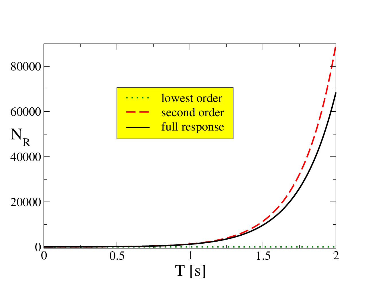
However, even for large values of the quadratic
approximation is a rather good one – provided that the duration of the
disturbance is not extremely large – as one can see in
Fig. 4.

Doing the same calculations for the corresponding right-dominated mode one finds as a result
where the remarkable agreement of coefficients of in
and of in as was already noticed
in Sec. III.3 is preserved for all orders in .
These terms fit the classical picture of particle transportation
through the leaky membrane where the particle flux is proportional
to the number of particles on the other side.
Again, expanding around up to second order yields exact
agreement with (82).
Accordingly, also outside the leaky cavity
particles are produced due to the dynamical Casimir effect, see also
Fig. 5.
Note that at least the quadratic answer is necessary to treat particle creation effects outside the leaky cavity. It is still valid that finite-temperature corrections will enhance the pure vacuum phenomenon of particle production by several orders of magnitude. (For a direct comparison see Fig. 7 in Sec. VIII.)
V.3 Further Remarks
We have derived a complete solution for the effective interaction Hamiltonian (62) which is valid to all orders in . As an illustration we consider a case outside our initial intentions where also assumes large values, e.g. . In this case the arguments of the hyperbolic functions in (V.2) and (V.2) will receive an imaginary part. The arising imaginary parts of cancel as they have to because is a physical observable. Thus one finds that if the velocity parameter exceeds the critical value the particle occupation number of the resonance modes versus the vibration time will exhibit oscillations. Of course, for the case of a nearly perfectly reflecting mirror inside this scenario is completely unrealistic since then will be relatively small. However, this case is not at all academic: If the label stood for a left-dominated mode – which is the case we excluded in our considerations so far and whose equivalent for ideal cavities has been considered in dalvit – may very well become large, since would then be of .

Similar oscillations of the particle number were also found in the case of strong inter-mode coupling in an ideal cavity dalvit.
Note that with this also leads to an upper bound for the internal mirror transmittance above which (corresponding to a highly transparent mirror) one finds oscillations that correspond to inter-mode coupling rather than to system-reservoir coupling. From another perspective this phenomenon could also be envisaged as follows: Starting with an ideal cavity whose original dimensions do not permit inter-mode coupling one can insert a highly transparent mirror (). This mirror in turn detunes the ideal cavity in such a way that it now permits inter-mode couplings as well.
It is remarkable that in Fig. 6 the phase of the two modes is shifted: When is at its maximum, then is at its minimum and vice versa. This fits nicely with the picture of mode hopping mediated by the inter-mode coupling . One even observes a decrease of the particle number in the -mode for small times. When defining an effective temperature finitetemp this would correspond to an effective cooling of the -mode. An extreme case of this consideration would be the limit of no squeezing, i.e. . This would correspond to the possibility (see also Sec. II.5) of not fulfilling the squeezing but the velocity resonance condition. Performing the limit everywhere in equations (V.2) and (V.2) one would find pure oscillations of the particle numbers and no exponential growth at all. This case is therefore counterproductive for an experimental verification. Note however, that this is different for the case of -coupling. The consistency with the earlier results leads to the conclusion that our approach was justified and the full response function should describe the rate of particle production correctly within the RWA.
Please note that the described procedure also holds for more than just two coupling modes: if one has e.g. modes fulfilling the resonance conditions given in Sec. II.5, the formalism still holds and one will have to define a dimensional vector . Of course then creation and annihilation operators of these resonance modes will be contained in the Hamiltonian and therefore also as well as will be by matrices. The calculations will simply become more involved but can certainly be performed, e.g. by means of computer algebra systems.
VI Detuning
So far we did assume an exact fulfillment of the resonance conditions, i.e. the vibration of the left cavity wall did match exactly twice the fundamental resonance frequency . However, in real situations one will of course have to deal with deviations from this desired external frequency since it will not be possible to match it with arbitrary precision. In addition, the back-reaction of the created quanta might cause the external vibration frequency to change.
Consequently, we will now discuss the detuned situation – where assumes slightly off-resonant values. For a review of detuning effects see e.g. leakydodonov; dalvit; dodonovdetuned. It has been shown in the literature that there exist threshold values for the detuning, above which the exponential creation of particles disappears.
Unfortunately the RWA used in our previous considerations cannot simply be generalized to this situation. For a slight deviation from the resonance conditions in equations (49) and (54) the terms with time-ordering – see section II.5 – are no longer negligible in this way.
We will consider slightly off-resonant situations, where the external vibration frequency does not match the fundamental resonance exactly
| (128) |
where denotes a small (dimensionless) deviation . However, if one considers such a variance it is only consequent to include a possible discrepancy of the coupling resonance as well, cf. dodonovdetuned
| (129) |
where denotes the deviation of the coupling right-dominated mode from the -coupling resonance condition with the fundamental resonance mode. We will adapt the multiple scale analysis (MSA) as proposed in dalvit to our scenario of a leaky cavity, see also dodonovdetuned. For this purpose we restrict to the results, since the steps in dalvit; dodonovdetuned can strictly be followed – see also appendix A. The main difference in these considerations is that we use the eigenfunction system of subsection II.3 instead of those of an ideal cavity and that we assume the additional deviation (129) – see also dodonovdetuned.
In analogy to subsection V.1 one obtains a matrix governing the time evolution of the ladder operators
The creation of quanta will only be exponential – and thus noticeable – if at least one of the eigenvalues of this matrix
does have a positive real part. Note that the slight disagreement between the above matrix and the one given in Ref. dodonovdetuned is caused by the usage of a different phase ( instead of ). With the abbreviations
and
the eigenvalues of the above matrix read (cf. dalvit; dodonovdetuned)
| (137) |
As a consistency check we may set where the eigenvalues reduce to the ones given in Eq. (V.1). On the other hand, for one recovers the usual result of pure squeezing in an ideal cavity .
Note that in contrast to dalvit; dodonovdetuned the inter-mode coupling and thus the parameter is very small . This enables us to expand the quantities and into powers of . The condition for a real eigenvalue reads
| (138) | |||||
Since is supposed to be small one obtains a significant contribution only if and also in this case merely in the immediate vicinity of the critical value . Consequently, the presence of an internal mirror of moderate quality do not drastically modify the threshold
| (139) |
for exponential particle creation. However, we would like to emphasize that the shifts of the eigenfrequencies of the cavity due to the partly permeable internal wall must be taken into account, see also section IX below.
VII Summary
We have considered a massless scalar quantum field inside a leaky cavity modeled by means of a dispersive mirror. For the case of the lossy cavity vibrating at twice the fundamental resonance frequency we derived an effective Hamiltonian using the rotating wave approximation. Within the framework of response theory the magnitude of particle creation due to the dynamical Casimir effect was calculated. Furthermore we deduced the corresponding master equation via applying the Born-Markov approximation. We found a discrepancy to the master equations used so far (see leakydodonov) to describe oscillating leaky cavities. We also applied a non-perturbative approach for the explicit calculation of the time evolution starting from the effective Hamiltonian. All these methods were found to lead to consistent results. In addition, the effects of a detuned external vibration frequency need to be taken into account.
It turned out that for the case of moderately low transmission coefficients (or sufficient quality factors) the rate of created particles is almost the same as for ideal cavities. The squeezing of the fundamental resonance mode as well as the strong enhancement of particle production due to the dynamical Casimir effect are preserved in the presence of transparent mirrors.
VIII Discussion
In order to illustrate reasonable magnitudes let us specify the relevant parameters: A cavity with a typical size of cm would have a fundamental resonance frequency of GHz i.e., the corresponding coupling right dominated mode must have a frequency of about GHz. According to Ref. leakydodonov we assume a dimensionless vibration amplitude . Consequently, in order to create a significant amount of particles one would have to sustain the external oscillations over an interval of several milliseconds. At room temperature K one finds the initial particle occupation numbers to be and . Using the above values the squeezing parameter determines to .
As the quality factor of a resonator is defined as jackson
| (140) |
one finds as a classical estimate yields for our system
| (141) |
denotes the transmission amplitude through the internal dispersive mirror and was defined in Sec. II. Assuming a -factor of leakydodonov (and references therein) this would imply for the corresponding perturbation parameter . With these values, a reasonable velocity parameter could be given by .
The particle content of the leaky cavity is depicted in
Fig. 7.

IX Conclusion
According to the above considerations it is necessary to vibrate several milliseconds in order to produce measurable effects. As already stated, a cavity at finite temperature might even be advantageous – provided the cavity is still nearly ideal at its characteristic thermal wavelength. However, even after only one millisecond ( periods) a classical estimate based on a quality factor of would indicate drastic energy losses. On the other hand, our calculations based on a complete quantum treatment show that the effects of losses are almost negligible compared to the rate of particle creation as long as . This leads to the conclusion that lower cavity quality factors than proposed in leakydodonov, e.g. [implying ] would already completely suffice to justify our approximations schaller. Such quality factors are within the reach of the current experimental status. Of course our calculations are based on the assumption that the larger cavity – including both the reservoir and the leaky cavity – is perfectly conducting. The error made by this presumption is of and therefore certainly negligible. Consequently, the experimental verification of the dynamical Casimir effect could be facilitated by a configuration where the vibrating cavity is enclosed by a slightly larger one as is demonstrated in Fig. 8.

X Outlook
X.1 Multi-Mode Coupling
In section II.5 we assumed that only one of the right-dominated modes fulfills the resonance condition for the velocity Hamiltonian, i.e., exactly two modes are coupled. If, however, the reservoir cavity becomes larger, the spacing between different levels of its spectrum decreases so that eventually more than just one right-dominated mode begin to couple – at least within the range of detuning. In this case the effective velocity Hamiltonian would constitute a sum of single two-mode coupling Hamiltonians as the one in Eq. (58) – but accounting for different right modes , , etc. As we have observed in Fig. 4 in Sec. V.2, the quadratic answer is completely sufficient for reasonable values of . Inserting the aforementioned sum of Hamiltonians into the quadratic answer one observes that the mixing terms vanish. Since the effective velocity Hamiltonian only contains odd powers of the creation and annihilation operators per mode, one can only obtain a non-vanishing trace if it involves two operators of the same (right) mode. Therefore the quadratic answer also decomposes into a sum of contributions each accounting for one right-dominated mode. Hence we expect the general structure of to persist – just substitute in the leading contributions44 4 Of course, multi-mode coupling can also be taken care of by the non-perturbative approach of Sec. V. The required effort, however, will increase very fast, since the corresponding matrix grows with the number of coupling modes.. In order to ensure the applicability of the perturbative treatment the number of coupling right-dominated modes has to be small enough to satisfy .
Typically the spacing between two neighboring right-dominated modes is of , i.e., the inverse of the characteristic length of the reservoir. On the other hand, the width of the resonance peak is of . Consequently, if the duration of the disturbance (1 ms) exceeds the characteristic length of the reservoir (which is the case for m) then is certainly small enough.
X.2 Electromagnetic Field
So far, we have considered a noninteracting, massless, and neutral scalar field. The next step could be to extend the calculations to the electromagnetic field. In this case several new difficulties arise:
- 1.
The boundary conditions cannot just simply be described by Dirichlet (or Neumann) conditions. Especially for moving walls their form will be more complicated due to Ampere’s law (mixing of and ).
- 2.
As the electromagnetic field is a gauge theory, one has to eliminate the unphysical degrees of freedom in order to quantize it. Again, for dynamic external conditions this requires special care, see e.g. quantumrad.
- 3.
The different polarizations of photons need to be taken into account which are of special interest concerning the fulfillment of the resonance conditions.
According to jackson the eigenmodes of the stationary cavity can be divided into TE and TM modes. For several cavities (rectangular, cylindrical, spherical) the eigenfrequencies are well-known. This enables one to determine the squeezing part of the interaction Hamiltonian.
In order to deduce the velocity Hamiltonian it will be necessary to
find an appropriate model for the dispersive mirror. This can be
achieved by using a thin dielectric slab with a high
permittivity: . As has been
shown for a stationary system in scully this leads to a similar
eigenvalue equation as (28).
For the detection of the created field quanta some detecting device will have to be placed inside the cavity, e.g. an atom. However, the detector will always influence the created field as well. A simple approach for the modeling of a two-level system has been provided in dodonov3; dodonov5. In addition, the non-adiabatic parametric modulation of the atomic Lamb shift – as has been considered in lambversuscasimir – must be taken into account, since it will cause excitations of the atom as well.
Note that the induced quantum field will also excite the internal degrees of freedom of the cavity mirrors – an alternate description of losses should therefore also take the energy dissipation of the losses within the mirrors into account, see e.g. leakylaw.
Future work combining all these effects is of immense importance regarding experiments on quantum radiation using the dynamical Casimir effect.
XI Acknowledgments
The authors are indebted to A. Calogeracos for fruitful discussions. R. S. acknowledges financial support by the Alexander von Humboldt foundation and NSERC. G. P. acknowledges financial support by BMBF, DFG, and GSI.
Appendix A Multiple Scale Analysis
Starting with the Lagrangian (5) it is straightforward to show that the field operator fulfills a modified wave equation
| (142) |
If one now follows dalvit by introducing ladder operators via the expansion
| (143) |
where
| (144) | |||||
| (145) |
one can derive a time evolution equation for the coefficients . Using the properties (7) of the eigenfunctions one obtains
where and in our scenario. The antisymmetric coupling is defined via
| (147) |
and is therefore related to the geometry factor via . Note that compared to dalvit the last line in (A) constitutes an additional term, since in our scenario the coupling between different modes may depend on the cavity parameters, see also equation (34). However, this difference is of minor relevance, since all these terms are accompanied by a factor of . If one assumes periodic oscillations of the cavity , these terms can be neglected if the amplitude is small. (The auxiliary function is chosen to meet the continuity conditions on , see also dalvit.) Consequently, one can expand (A) in powers of to yield
| (148) | |||||
This equation completely resembles the one found in dalvit. Note however, that we have to use the shifted eigenfrequencies and the eigenfunctions for leaky cavities. An approximate solution – for a more detailed discussion see dalvit – can be obtained via introducing a new time scale and inserting the formal expansion
| (149) |
with the unknown functions into equation (148). Finally, one has to sort in powers of . To lowest order one finds a free harmonic oscillator which can be solved by
| (150) |
The next order terms (proportional to ) yield a driven harmonic oscillator equation for with the eigenfrequency
In order to keep the expansion (149) convergent, above oscillator must not be at resonance. Consequently, all terms proportional to – with being the particular mode of interest – on the right hand side have to cancel. By imposing these conditions for the mode and for the coupling mode and inserting the frequency deviations
| (152) | |||||
| (153) |
one finds four linear and coupled evolution equations for the coefficients , , , and . These equations are – apart from the different couplings and the additional deviation – virtually identical with those presented in dalvit. Having applied the modified phase transformations
| (154) | |||||
| (155) | |||||
| (156) | |||||
| (157) |
it is straightforward to rewrite these equations in matrix form.
where
The quantities have been introduced for convenience
| (168) | |||||
| (169) | |||||
| (170) | |||||
References
- (1) H. B. Casimir, Proc. K. Ned. Akad. Akad. Wet. 51, 793 (1948).
- (2) M. Bordag, Quantum Field Theory Under the Influence of External Conditions, (Teubner, Stuttgart, 1996); The Casimir Effect 50 Years Later, (World Scientific, Singapore, 1999).
- (3) M. T. Jaekel and S. Reynaud, J. Phys. I (France) 2, 149 (1992); Phys. Lett. A 167, 227 (1992); J. Phys. I 3, 1093 (1993); Phys. Lett. A 180, 9 (1993); Phys. Lett. A 172, 319 (1993); J. Phys. I (France) 3, 1 (1993); J. Phys. I (France) 3 339 (1993); Quant. Semiclass. Opt. 7, 499 (1995).
- (4) G. Bressi, G. Carugno, R. Onofrio, and G. Ruoso, Phys. Rev. Lett. 88, 041804 (2002); U. Mohideen and A. Roy, Phys. Rev. Lett. 81, 4549 (1998); S. K. Lamoreaux, Phys. Rev. Lett. 78, 5 (1997).
- (5) G. Plunien, R. Schützhold, and G. Soff, Phys. Rev. Lett. 84, 1882 (2000); R. Schützhold, G. Plunien, and G. Soff, to appear in Phys. Rev. A.
- (6) J. Ji, H. Jung, J. Park, and K. Soh, Phys. Rev. A 56, 4440 (1997).
- (7) M. Crocce, D. A. R. Dalvit, and F. D. Mazzitelli, Phys. Rev. A 64, 013808 (2001).
- (8) A. V. Dodonov and V. V. Dodonov, Phys. Lett. A 289, 291 (2001).
- (9) R. Golestanian and M. Kardar, Phys. Rev. Lett. 78, 3421 (1997).
- (10) A. Lambrecht, M. T. Jaekel, and S. Reynaud, Phys. Rev. Lett. 77, 615 (1996); Eur. Phys. J. D 3, 95 (1998).
- (11) P. C. Davies and S. A. Fulling, Proc. Roy. Soc. Lond. A 348, 393 (1976).
- (12) V. V. Dodonov, Phys. Rev. A 58, 4147 (1998); Phys. Lett. A 244, 517 (1998).
- (13) G. Schaller, R. Schützhold, G. Plunien, and G. Soff, Phys. Lett. A 297, 81 (2002).
- (14) R. Lang, M. O. Scully, and W. E. Lamb Jr., Phys. Rev. A 7, 1788 (1973).
- (15) J. Gea-Banachloche et al., Phys. Rev. A 41, 369 (1990).
- (16) G. Barton and A. Calogeracos, Ann. Phys. 238, 227 (1995); A. Calogeracos and G. Barton, Ann. Phys. 238, 268 (1995).
- (17) G. M. Salamone and G. Barton, Phys. Rev. A 51, 3506 (1995).
- (18) R. Schützhold, G. Plunien, and G. Soff, Phys. Rev. A 57, 2311 (1998).
- (19) R. Schützhold, Phys. Rev. D 63, 024014 (2001).
- (20) C. K. Law, Phys. Rev. A 49, 433 (1994); Phys. Rev. A 51, 2537 (1995).
- (21) Y. Wu, M.-C. Chu, and P. T. Leung, Phys. Rev. A 59, 3032 (1999).
- (22) R. Schützhold, G. Plunien, and G. Soff, Phys. Rev. A 58, 1783 (1998).
- (23) V. B. Braginsky and F. Ya. Khalili, Phys. Lett. A 161, 197 (1991).
- (24) V. V. Dodonov, A. A. Klimov, and D. E. Nikonov, J. Math. Phys. 34, 2742 (1993).
- (25) V. V. Dodonov, J. Phys. A 31, 9835 (1998).
- (26) V. V. Dodonov and A. B. Klimov, Phys. Rev. A 53, 2664 (1996).
- (27) V. V. Dodonov, A. B. Klimov, and A. E. Nikonov, Phys. Rev. A 47, 4422 (1993).
- (28) V. V. Dodonov, Phys. Lett. A 207, 126 (1995).
- (29) V. V. Dodonov, J. Phys. A 32, 6711 (1999).
- (30) D. A. R. Dalvit and P. A. Maia Neto, Phys. Rev. Lett. 84, 798 (2000); P. A. M. Neto and D. A. R. Dalvit, Phys. Rev. A 62, 042103 (2000).
- (31) L. Mandel and E. Wolf, Optical Coherence and Quantum Optics, (Cambridge University Press, Cambrigde, 1995).
- (32) E. Fick and G. Sauermann, Quantenstatistik Dynamischer Prozesse, (Harri Deutsch, Frankfurt/Main, 1983); The Quantum Statistics of Dynamic Processes, (Springer, Berlin, 1983).
- (33) M. Freyberger et al., Quantized Field Effects, in Atomic, Molecular & Optical Physics Handbook, edited by G. W. F. Drake, (AIP Press, Woodbury, New York, 1996).
- (34) V. V. Dodonov and M. A. Andreata, J. Phys. A 32, 6711 (1999).
- (35) J. D. Jackson, Classical Electrodynamics, (Wiley, New York, 1999).
- (36) C. K. Law, T. W. Chen, and P. T. Leung, Phys. Rev. A 61, 023808-1 (2000).
- (37) N. B. Narozhny, A. M. Fedotov, and Yu. E. Lozovik, Phys. Rev. A 64, 053807 (2001).