Gravitational decoherence of atomic interferometersThanks: Unité mixte du CNRS, de l’École Normale Supérieure et de l’Université Pierre et Marie Curie.Thanks: Unité propre du CNRS, associée à l’École Normale Supérieure et à l’Université Paris XI Orsay.
Abstract
We study the decoherence of atomic interferometers due to the scattering of stochastic gravitational waves. We evaluate the ‘direct’ gravitational effect registered by the phase of the matter waves as well as the ‘indirect’ effect registered by the light waves used as beam-splitters and mirrors for the matter waves. Considering as an example the space project HYPER, we show that both effects are negligible for the presently studied interferometers.
pacs
03.65.YzDecoherence; open systems; quantum statistical methods and 03.75.-bMatter waves and 04.30.-wGravitational waves: theory1 Introduction
The idea that spacetime fluctuations could play a universal role in the transition from quantum to classical physics has been proposed by a number of authors. Already present in the Feynman lectures on gravitation Feynman99; Feynman63, it was more thoroughly developed and popularized for instance in Karolyhazy66; Diosi89; Penrose96; Ellis98. An important argument in favor of such an idea is that the Planck mass, i.e. the mass scale built on the Planck constant , the velocity of light and the Newton constant , has a value g lying on the borderland between microscopic and macroscopic masses. In other words, microscopic masses could be characterized as masses for which the associated Compton length is larger than the Planck length m whereas macroscopic masses would correspond to a Compton length smaller than the Planck length .
Clearly, this dimensional argument is not by itself sufficient to reach definitive conclusions. It can be hoped that the existence of fundamental spacetime fluctuations, with a length scale determined by , may be revealed by long-term diffusion effects in the same manner as microscopic molecular motion is revealed by Brownian motion. It has for instance been proposed that intrinsic spacetime fluctuations could be observed through a decoherence effect which might be visible with matter-wave interferometers Percival97; PercivalS97; Power00; Amelino99; Amelino00. The effect has not been seen in existing matter-wave interferometers Peters99; Peters01; Gustavson00. More sensitive instruments are being developed, like the atomic interferometer HYPER designed to measure the Lense-Thirring effect in a space-borne experiment, and it is important to estimate the ultimate decoherence due to fundamental spacetime fluctuations for such an instrument Hyper00.
The aim of the present paper is to give quantitative answers to this question by considering the decoherence mechanism associated with the scattering of gravitational waves present in our celestial environment. These gravitational waves are the intrinsic fluctuations of spacetime predicted by general relativity Misner. The latter theory can be used as an accurate effective theory of gravitation for all frequencies ever explored in experiments Will90; Damour94. The gravitational waves are the intrinsic field fluctuations predicted by the linearized form of the theory Weinberg65; Grishchuk77; Zeldovich86. This linearized form is widely used for studying propagation of gravitational waves and their interaction with the presently developed interferometric detectors Schutz99; Maggiore00; Ungarelli00.
In the present paper, we will study the decoherence of an atomic interferometer due to its interaction with the stochastic background of gravitational waves emitted by unresolved sources in our galaxy or its vicinity Hils90; Giazotto97. These waves dephase differently the matter-waves on the two interfering paths as well as the light-waves used to build up beam-splitters and mirrors in atomic interferometers AtomInt97. When averaged over the integration time of the measurement, the differential dephasing results in a loss of contrast of the interference fringes. We will use the remaining fringe contrast to characterize the decoherence and write it in terms of the geometry of the interferometer and of the statistical function describing the gravitational environnement.
In this approach, decoherence will be understood as resulting from a phase dispersion due to the unobserved degrees of freedom of the gravitational environnement. To be more precise, gravitational waves with frequencies in the detection window of the interferometer have to be interpreted as signals while frequencies outside the detection window are ignored. In a typical situation, the detection window corresponds to frequencies smaller than the inverse of an averaging time. The integration over frequencies outside the detection window can thus be identified with the trace over the environnemental degrees of freedom usually considered in theoretical studies of decoherence Zeh70; Dekker77; Zurek81; Zurek82; Caldeira83; Caldeira85; Joos85; Raimond01. The phase dispersion approach used in the present paper is known to be equivalent to the other approaches to decoherence Imry90 and it is obviously well adapted to the description of interferometers where the phase is the natural variable.
We will show in this paper that the scattering of gravitational background does not lead to an appreciable decoherence effect for the atomic interferometers presently studied, HYPER being chosen as the typical example. Incidentally, this means that atomic interferometers will not have their interference fringes destroyed by this decoherence mechanism. This answer has to be contrasted with recently published results which prove that the scattering of stochastic gravitational waves present in our galactic environment is the dominant, and extremely efficient, decoherence mechanism for macroscopic motions, say the planetary motion of the Moon around the Earth Reynaud01; Reynaud02. This contrast is easily explained by the already evoked dimensional argument : gravitational decoherence effects are likely to be more efficient for macroscopic masses than for microscopic objects. In particular, the mass of the Moon is larger than Planck mass by orders of magnitude whereas the microscopic entities used as spacetime probes in atomic interferometers have their mass much smaller than Planck mass. However, as already stated, this simple scaling argument is not by itself sufficient to answer quantitative questions about the decoherence rates. In the following, we will give precise estimations of the decoherence effect which depend not only on the mass of the atoms, but also on their velocity, on the geometry of the interferometer and on the noise spectrum characterizing the gravitational background in the relevant frequency range.
2 Gravitational backgrounds
A first step is to characterize the fundamental fluctuations of spacetime and their effect on the motion of matter. Although a complete quantum theory of gravity is not available, it is possible to describe spacetime fluctuations in our environment. At the frequencies of experimental interest, which are much smaller than Planck frequency, they are identified Reynaud01; Reynaud02 as the stochastic backgrounds of gravitational waves currently studied in relation with the development of gravitational wave detectors Schutz99.
The effect of gravitational perturbations may in principle be described in a manifestly gauge-invariant manner. In the present paper, we will adopt the common strategy of studies of gravitational waves : admitting that this point can be dealt with, we then chose a specific gauge, namely the transverse traceless (TT) gauge with metric perturbations differing from zero only for purely spatial components ( stand for the spatial indices whereas represents the temporal index). Then gravitational waves are conveniently described through a mode decomposition Blanchet00 :
| (1) |
Any Fourier component is a sum over the two circular polarizations :
| (2) |
Gravitational waves correspond to wavevectors lying on the light cone and they are transverse with respect to this wavevector :
| (3) |
The gravitational polarization tensors are obtained as products of the polarization vectors well-known from electromagnetic theory. When necessary, we will chose the following representation for the unit vector along the propagation direction of the gravitational wave and the corresponding polarization vectors :
Spatial vectors are written as bold letters. Note that reality conditions for the perturbation metric are read :
| (12) |
We use the natural caracterization of the stochastic background in terms of the spectral density of strain fluctuations of the metric. For simplicity, we consider the case of gaussian, stationary, unpolarized and isotropic backgrounds :
| (13) |
The general case could be dealt with by considering arbitrary correlations between amplitudes and . This would allow one to take into account polarized or anisotropic backgrounds, as is necessary for a thorough analysis of the galactic background, as well as non stationnary fields appearing in some cosmological models Grishchuk77; Grishchuk90.
Gravitational backgrounds are usually written in terms of one metric component (say , but the result would be the same for other components due to the isotropy assumption) at a fixed spatial position (say , but the result would be the same for other positions due to the stationarity assumption) as a function of time . They are thus described by the spectral density of strain fluctuations considered in most papers on gravitational waves detectors Maggiore00 :
| (14) |
This noise spectrum, written in the TT gauge, is not gauge invariant. This is not a problem since only gauge invariant quantities will be computed in the following. It follows from equations (14,2) that is obtained by integrating over the momenta which correspond to a given frequency :
| (15) |
We have denoted by the averaging over spatial directions of wavevectors at a given frequency. Using the fact that gravitational wavevectors lie on the light cone and the simplifying assumptions already described, we inverse the preceding relation to obtain :
| (16) |
In this paper, we will consider the binary confusion background
describing gravitational waves emitted by unresolved binary systems in
our galaxy or its vicinity. This background is represented for example
on figure (1) of reference Schutz99. It relies on the laws of
physics and astrophysics as they are known in our local celestial
environment. In particular, it depends on the statistical repartition
of binary systems in the sky. In the frequency range of interest,
which is discussed in more detail below, the binary confusion
background dominates other sources of stochastic gravitational waves,
in particular those associated with cosmological contributions. Note
that this frequency range, between Hz and mHz, corresponds to
frequencies much smaller than the detection window of VIRGO and other
ground-based optical interferometers but roughly of the same order as
the frequencies in the detection window of the space-borne project
LISA
11
1
Informations on the ground-based GW detectors may be found
on the Web sites; VIRGO : http://www.virgo.infn.it/ ; GEO :
http://www.geo600.uni-hannover.de/ ; LIGO :
http://www.ligo.caltech.edu/ ; TAMA :
http://tamago.mtk.nao.ac.jp/tama.html ; ACIGA :
http://www.anu.edu.au/Physics/ACIGA/ .
Informations on the space-borne interferometer LISA may be found on
the Web sites at NASA : http://lisa.jpl.nasa.gov/ and ESA :
http://sci.esa.int/home/lisa/ ..
The properties of the gravitational bath may also be characterized by an effective number of gravitons per mode (the precise relationships between and are given in the last section). It is worth noting immediately that this number is extremely large, so that the gravitational environment corresponds to the limit of high-temperature classical fluctuations. As a consequence, the vacuum fluctuations of the gravitational field Grishchuk90, which have been shown to lead to ultimate fluctuations of geodesic distances of the order of Planck length Jaekel94; Jaekel95QSO; Jaekel95AP, are ignored in the present paper. We also note that, as the number of unresolved binary systems contributing to the binary confusion background is large and as these sources are independent of each other, it appears quite safe to consider that the gravitational background obeys gaussian statistics (this might not be true for cosmological contributions).
In order to discuss our main results in the end of the present paper, we will use the fact that the binary confusion background corresponds to a nearly flat function in the frequency range Hz. This means that the gravitational noise spectrum is quasi-thermal at such frequencies and entails that the decoherence mechanism can be interpreted as a Brownian-like diffusion process. We will estimate quantitatively the quantity playing the role of the diffusion coefficient and show that it does not lead to an appreciable decoherence effect for atomic interferometers like HYPER.
3 Gravitational decoherence
Now we want to quantify the effect of the previously discussed gravitational waves on the coherence properties of an atomic interferometer. In the present section, we present a detailed discussion of this effect which could basically be schematized as follows : coherence of the interference fringes is preserved if and only if the differential phase perturbation between the two arms is controlled to a level much better than .
When propagating in spacetime, the atomic probe field registers curvature fluctuations. The main effect of the perturbation is described by the eikonal approximation, valid for wavevectors of the gravitational wave much smaller than wavevectors of the probe field. This effect is characterized as a dephasing of the probe field, evaluated at a fixed spatial position (say ) as a function of time . At the lowest order, the dephasing is linear in the metric and can be decomposed over the gravitational wave modes :
| (17) |
At the moment, are time-dependent coefficients which depend on the geometry of the interferometer. These coefficients will be explicitly written in the forthcoming sections but we already know that they satisfy the reality conditions :
| (18) |
For a stationary, isotropic and unpolarized background, the correlation function for the dephasing is deduced :
| (19) |
The gravitationally induced dephasing is not always a stationary noise. Here, we will focus our attention on situations where it is stationary or quasi-stationary and where the correlation function is simply represented by a noise spectrum :
| , | (20) |
In fact, we have supposed that the amplitudes are only slowly dependent functions of time and, furthermore, we have used the reality condition (18). The equation thus obtained means that the stochastic dephasing has a noise spectrum equal to the product of two factors, the gravitational noise spectrum and the apparatus response function which depends on the geometry of the apparatus.
As mentioned earlier, the analysis of decoherence should in principle take into account the detection strategy used in the interferometric measurement. In order to fix ideas, we will consider a simple strategy where the output of the interferometer, supposed to be linear in the variation of the dephasing , is averaged over an averaging time . This means that the signal, for instance the Lense-Thirring effect in HYPER experiment Hyper00, is contained in the averaged dephasing which is read in the frequency domain as :
| (21) |
In other words, the signal window is defined by a low-pass filter with a bandwidth . Now, the frequencies outside the signal window constitute an uncontrolled noise which may degrade the coherence of the interferometer if it is large enough.
In order to estimate this potential decoherence effect, we define the uncontrolled dephasing which is also the dephasing after a high-pass filter with the same bandwidth :
| (22) |
We then consider the visibility of the fringes which is the mean value of the exponential of the uncontrolled phase noise :
| (23) |
As we have supposed the gravitational background to obey the gaussian statistics, the various dephasings are also gaussian stochastic variables. It follows that the visibility of the fringes may be expressed in terms of the variance of the uncontrolled noise :
| (24) |
Finally this variance is given by the following integral over frequency :
| (25) |
The last two equations are a fondamental result of this article. They quantitatively characterize the gravitational decoherence effect through the reduction of the fringe visibility . This visibility is the exponential of the phase noise variance. The latter is an integral over the whole frequency spectrum of a product of factors. Besides the gravitational noise spectrum and the apparatus response function which have already been discussed, there is a further factor, a high-pass filter with a cutoff , which defines uncontrolled noise as corresponding to frequencies outside the detection window. For simplicity, we have considered here a Lorentzian expression associated with a simple averaging strategy. Note that the filter may help us to regularize potential infrared divergences in the forthcoming calculations. We shall see later on that this is not necessary for the situations considered in this paper and that the results are essentially independent of the cutoff. Note also that it would be easy to replace the Lorentzian filter by more sophisticated expressions corresponding to different signal detection strategies.
As it is usual in decoherence theory, the remaining coherence, here the visibility , is the exponential of a noise variance, the variance of the uncontrolled noise. From the point of view of the interferometrist, this expression has a quite clear expression : the gravitational perturbation dephases differently the waves in the two arms, and the fringe contrast is appreciably degraded if and only if the resulting variance is of the order or greater than unity. At this point, it is worth emphasizing that the same result would have been obtained through more formal approaches of decoherence with the uncontrolled noise frequencies thus interpreted as the degrees of freedom of the environment (see for example Imry90 for a more detailed discussion of this point).
Expression (25) is valid for a gaussian, stationary, isotropic and unpolarized background. The numerical factor is a factor arising from angular averaging for an isotropic and unpolarized background. As already mentioned, generalization to anisotropic, polarized and non stationary background is possible. Even non gaussian noise can in principle be dealt with by developping the fringe visibility in cumulants of the stochastic noise. However, these refinements would not change the main conclusion of the paper, namely that the gravitational decoherence is not efficient for presently studied atomic interferometers such as HYPER. The next sections are devoted to explicit calculations of the apparatus function for such an interferometer.
4 Atomic interferometer with a Mach-Zehnder geometry
In order to smoothly introduce the more technical parts of our evaluations, we first consider in this section an hypothetical atomic interferometer with the same Mach-Zehnder geometry as HYPER but where optical elements, beam splitters and mirrors, would be built up from massive and motionless material pieces. A more realistic description of HYPER with optical elements built up on stimulated Raman processes is presented in the next section.
The Mach-Zehnder geometry is represented on figure (1). The atomic matter-waves are supposed to follow their classical trajectories. Equivalently, they obey the propagation equation of a scalar field with a wavevector and the dephasing is the first-order effect of the gravitational perturbation of the associated lagrangian. Then, the dephasing evaluated on a closed loop is gauge-invariant, as soon as conservation of the energy-momentum tensor is properly taken into account Landau. This raises specially delicate problems for the description of beam splitters and mirrors in the interferometer.
In the present section, we solve these problems by using the method commonly adopted for the description of optical interferometers Grishchuk88; Hellings92 : the treatment is largely simplified when optical elements such as beam splitters and mirrors are described as heavy objects initially at rest and gravitational waves described in the TT gauge. In this gauge indeed, gravitational waves have no effect on massive objects at rest. And objects with a large mass may be considered as staying at rest when initially at rest, since the momentum transfered by the field upon scattering does correspond to a negligible velocity change. This implies that the effect of gravitational waves on optical elements can be ignored throughout the calculation. This treatment is certainly an approximated one. In particular, the assumptions just discussed entail that the interferometer is at rest. This is obviously not the case for HYPER which is orbiting around the Earth, this motion being important for the analysis of the signal associated with the looked for Lense-Thirring effect Hyper00. However this motion may be disregarded in the discussion of decoherence in the present paper. In the present section, we build up our calculations on this approximation.
Now we write the dephasing obtained from the geodesic deviation equation for the probe field :
| (26) |
This equation is written in the eikonal approximation where the wavevector of the gravitational waves is much smaller than the wavevector of the probe field Mashhoon80. The integral (26) is taken along the unperturbed geodesic path of the probe with the coordinate time used as an affine parameter; denotes the time of propagation along the path, and is the reduced wave vector :
| (27) |
We then deduce the coefficients which characterize the sensitivity of the dephasing to the gravitational wave :
| (28) |
These coefficients are time-independant, due to the stationarity assumption and to the fact that we have supposed the interferometer to be at rest.
 |
As a consequence of the preceding discussions, the global dephasing of the interferometer is obtained by adding the contributions of the free propagation segments :
| (29) |
We ignore any dephasing of the probe field associated with scattering on the beam splitters. This point will be discussed in more details in the next section.
For simplicity, we consider the interferometer to have a rhombic geometry with the aperture angle and the length of each side. The latter quantity is related to the time of flight and the modulus of the atomic velocity :
| (30) |
We suppose the interferometer to lie in the plane and write the coordinates of its apexes in a manner exploiting the symmetry of the rhomb ( for all points) :
| , | |||||
| , | |||||
| , | |||||
| , | (31) |
We have used the stationarity to select a specific time. Then the reduced velocities are read :
| (32) |
We now evaluate the amplitude corresponding to the segment [AB] from equation (28). We restrict our attention to the non relativistic limit so that :
| (33) |
Using the symmetry of the rhomb, we then deduce the amplitude corresponding to the sum over the four segments :
| (34) |
where is the kinetic energy of the atom measured as a frequency. We finally get the apparatus response function :
| (35) |
where we have introduced the function :
| (36) |
We now come back to the phase noise variance (25) which determines the fringe contrast (24). This expression characterizes the decoherence of the atomic interferometer for an arbitrary gravitational noise spectrum , for example the spectrum describing the binary confusion background Schutz99; Maggiore00. As already mentioned, we see that this filter may help us to regularize potential infrared divergence of this spectrum, besides the factor which already cuts off low frequencies.
This discussion can be made more explicit by considering the specific case where the spectrum is constant in the domain relevant for evaluating the integral (25). Note that this is approximately the case for evaluating the effect of the binary confusion background for HYPER. As a matter of fact, the signal has to be integrated over an averaging time ranging between 1 day and 1 month. Such an averaging time corresponds to the frequency range 1-30Hz. In this frequency range, the binary confusion background dominates the other contributions, in particular cosmological ones, and it has a quasi-thermal spectrum. Hence, the integral (25) can be estimated, at least roughly, by replacing the frequency dependent noise spectrum by a constant. Since the binary confusion background decreases at higher frequencies, the result obtained in this manner has to be considered as an upper limit for the phase noise variance.
In this simple case, the integral (25) may be deduced from the following properties of the function :
| (37) |
so that :
| (38) |
Now, the time of flight of the atoms on the segment [AB] is of the order of 1.5 s in HYPER Hyper00 and the averaging time is much longer. This entails that the preceding formula may be simplified by taking the further limit :
| (39) |
with the result :
| (40) |
We note that is the geometrical characteristic of the interferometer which determines the difference between the two paths and plays the role of the classicality parameter entering usual expressions of decoherence rates Zurek81; Zurek82.
The cutoff is no longer present in the estimate (40). This argument may be laid down in a more general manner. High sensitivity measurements usually require long integration times so that the condition is met with the time of flight of the probe field in the interferometer. If the noise spectrum has such a low-frequency behaviour that no regularization of the integral is needed, then the variance of the phase noise may be evaluated by forgotting the filter :
| (41) |
If, furthermore, the spectrum is nearly flat in the frequency domain determined by the apparatus function , then the variance of the phase noise is simply the product of the constant value of by the integral of this apparatus function and the latter is obtained from :
| (42) |
Now we proceed to a numerical evaluation of the decoherence effect. We use the following numbers which correspond to HYPER with the choice of Cs atoms Hyper00 :
| (43) |
is the transverse velocity communicated to the atoms by the beam splitters and mirrors; it will be discussed in more details in the next section. Using the noise level in the frequency range of interest , we finally obtain the phase noise variance due to the dephasing of the atomic matter-waves in HYPER :
| (44) |
Clearly, the decoherence computed in this manner is completely negligible, and the fringe contrast is unaffected by the direct coupling of gravitational waves to atomic matter-waves.
5 HYPER-like interferometers
We have already noticed that, in the most sensitive presently studied atomic interferometers, optical elements are built up on stimulated Raman processes Peters01. As a consequence, the dephasing seen by the interferometer also picks up the gravitation perturbation of the lasers involved in these optical elements. In the present section, we give a precise evaluation of this ‘indirect’ effect and show that it largely dominates the ‘direct’ atomic effect studied in the preceding section. In order to fix the orders of magnitude, we will still consider the numbers corresponding to the project HYPER Hyper00.
The use of stimulated Raman processes to build up optical elements such as beam splitters or mirrors for atomic matter waves has been described in a number of papers (see for example Borde89; Borde92; Kasevich92; Weiss94; Storey94). In the stimulated Raman process, atoms interact with two counter-propagating lasers with slightly detuned frequencies and . The detuning is chosen so that the Raman process, absorption of one photon in one beam and stimulated emission of one photon in the other beam, is resonant with a transition between two hyperfine ground states. In contrast, the detuning between one-photon interaction and the intermediate excited state is sufficiently large so that spontaneous emission plays a negligible role. This also entails that the equivalent duration of the whole Raman process is so short that the Raman process can be considered as spatially and temporally localized. Besides the transition from one ground level to the other, the main effect of the Raman process is a momentum transfer between the field and atom. This momentum transfer has its direction along the transverse direction of the rhomb and it is responsible for the beam splitting effect with a change of transverse velocity of the atoms :
| (45) |
where is the nearly common value of the laser frequencies.
 |
The whole interferometer is sketched on figure (2) with the atomic and photonic paths now represented. Each momentum transfer is accompanied by a change of atomic ground state and the atoms are in the same state in the output beam as in the input one. This means that the amplitudes corresponding to the two arms are able to interference. However, the gravitational perturbation is now registered not only by the atomic matter-waves but also by the laser fields. As shown in the following, the ‘indirect’ photonic contribution even dominates the direct atomic one.
We will write the whole dephasing between the two arms as :
| (46) |
is the dephasing picked up by the atomic matter waves when they propagate along the linear segments [AB], [BD], [AC] and [CD] of the interferometer. It has already been calculated in the previous section. is the gravitational dephasing of the electromagnetic phases involved in the stimulated Raman processes. It can be written as a sum over the optical elements :
| (47) |
Internal phase factors, corresponding to evolution at the different frequencies of the two atomic ground states, do not appear in the final expression, due to a proper account of energy conservation. But the same energy conservation law enforces that the photonic phase is present : the change of momentum of the atoms on the beam splitters is just equal to the change of momentum of the field state.
We now evaluate the gravitational dephasing of the laser waves involved in the stimulated Raman process at beam splitter B. They are obtained as the effect of gravitational waves on the counter-propagating laser waves before the latter attain the atoms at point B. We use the simplifying assumption that the Raman process is instantaneous, so that the dephasing of the two lasers has to be evaluated at the same spatio-temporal point. The calculation is the same as for standard optical interferometers Grishchuk88; Hellings92 with optical paths described on the space-time diagram of figure (3). As in the preceding section, the macroscopic reference objects, that is the laser sources and mirrors reflecting photons, are supposed to be at rest initially and to stay at rest, thanks to their large mass.
 |
The coordinates of the point B are fixed as in the preceding section. The coordinates of the other apexes are displaced with respect to that of B in the direction of the axis which is the propagation direction of the lasers (see figure 2) :
| , | ||||
| , | ||||
| , |
We have introduced the notations for the time of flight of photons from the laser source L to the mirror M and for the time of flight of photons from the mirror M to the atom at B. The reduced velocities have simple expressions for photons :
| (49) |
If follows from the expressions (2) that all polarization factors involved in the evaluation of have the same simple form .
The dephasing is then deduced from a factor representing a decomposition in momentum space :
| (50) |
From now on, we neglect the difference between the two laser frequencies . We introduce a notation to represent the phase time of the mode at the point B. We also introduce the notations for the factors measuring the angle of propagation between gravitational and electromagnetic waves. Since these waves propagate at the same speed, potential resonances might occur in the limit of colinear propagation or , as shown by the appearance of the denominators in . In fact, these resonances do not occur because the numerators of the fractions and, also, the polarization factor vanish in this limit Mashhoon80.
We then perform the same evaluation for the other contributions, , and which are involved in the whole photonic dephasing (47). Assuming for simplicity that the geometry is the same for the four beam splitters and mirrors, these 4 terms only differ through a global phase and their interference leads to :
| (51) |
The phase-times , and are defined as from the phases of the gravitational mode at the spacetime points corresponding to the passage of the atom at corresponding optical elements.
The magnitude of the photonic dephasing is mainly determined by the laser frequency whereas the magnitude of the atomic dephasing was proportional to the frequency . Since the latter frequency is much smaller than the former, it is expected that :
| (52) |
We will see at the end of the present calculation that this is the case. As a consequence, the correlation between atomic and photonic dephasings will also have a negligible contribution. It follows that the phase noise variance (25) will be determined essentially by the photonic contribution :
| (53) |
Note that the two polarizations have the same contribution to the present result.
We use the function (36) to express the squared amplitudes :
| (54) |
and :
| (55) | |||||
These equations give the phase noise variance due to photons for an arbitrary noise spectrum .
In order to go further, we perform the same approximations as in the preceding section. We consider the case of a thermal bath with the noise spectrum constant over the frequency domain relevant for the integral (25). We focus our attention on the limit of a small and use the integral (42) as well as the further properties of the function :
| (56) |
| (57) |
has been defined so that the expression of has the same form as in (40); it is obtained from the auxiliary function which has the same structure as in (55) :
| (58) | |||||
The lengths are of the same order for atomic and photonic lines, but the velocity of light is much larger than the atomic velocity . Hence the atomic time of flight is much larger than the photonic ones and . It follows that is much larger than the other time parameter appearing in the function in the preceding equation, except for specific gravitational modes propagating along the segments of the atomic rhomb. Disregarding these exceptions which have a negligible contribution to the spatial mean values, we obtain a good approximation for the function :
| (59) |
Since the function no longer depends on the parameter , the equivalent photonic interaction time is simply :
| (60) |
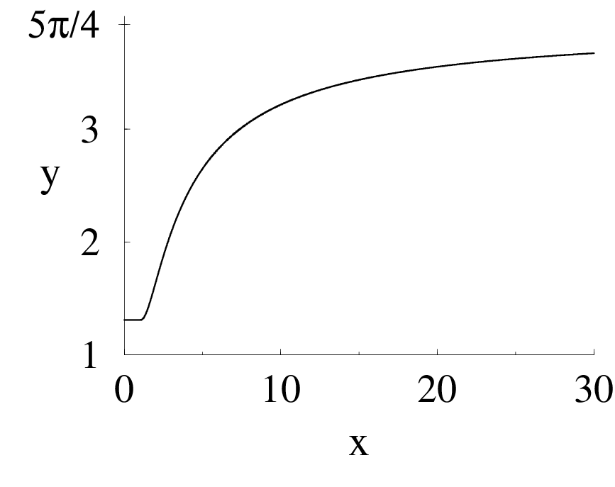
The numerical factor is a function of the ratio which can be obtained through a numerical integration :
The function is drawn on figure 4.
 |
Finally the phase noise variance corresponding to the photonic lines is essentially determined by the time of flight of photons between atoms and mirrors :
| (64) |
Using the numbers corresponding to HYPER :
| (65) |
we get the following estimation of the phase noise variance associated with photonic lines :
| (66) |
This indirect contribution due to the gravitational perturbation of electromagnetic waves is much larger than the direct effect of gravitational waves on atomic matter waves. This result was anticipated from the fact that the laser frequency is much larger than the corresponding atomic quantity . It was however necessary to perform the whole calculation to reach an unambiguous conclusion, because the variance also depends on the times of exposition of photons to the gravitational interaction, these times and being smaller than .
The final result proves that the decoherence of HYPER-like interferometers is dominated by the photonic contribution. In other words, as far as the coupling to gravitational waves is concerned, such interferometers essentially behave as optical detectors with a readout mediated by atomic waves. A second important consequence of our result is that the photonic contribution to decoherence, though much larger than the atomic one, is still completely negligible. Hence, the fringe contrast of HYPER is unaffected by the scattering of gravitational waves.
It is worth explaining this result in more details in terms of spectra. To this aim, we come back to the expression (25) where the variance is the integral of a phase noise spectrum . We then simplify this expression by performing the already discussed approximations : is considered as constant and the crossed terms in the squared amplitudes are disregarded. Keeping only the square terms we get a typical dependence :
| (67) |
where is one of the times of flight involved in equation (55). The phase noise spectrum has a magnitude of the order of and a bandwidth of the order of which lead to an integral of the order of . This simple estimate fits the result (64) obtained through a more rigorous calculation.
Now the phase noise level may be measured as an equivalent vibration noise for the mirrors reflecting the lasers. This equivalent noise, written in terms of the position of a mirror, is approximated as :
| (68) |
We have again used the numbers of HYPER with nearly equal to 1m. This corresponds to a noise level which is far beyond the vibration noise level which is the target of the HYPER instrument. This discussion confirms that the phase noise induced by the scattering of gravitational waves is completely negligible in HYPER-like interferometers. In particular, it shows that this fundamental spacetime noise is smaller than the residual phase noise corresponding to mechanical vibrations of the mirrors.
6 Discussion
It had been suggested that atomic interferometers could be sensitive to a decoherence effect stemming from intrinsic spacetime fluctuations. In the present paper, we have studied the effect associated with the scattering of gravitational waves, which we expect to be the dominant source of spacetime fluctuations in the frequency domain of interest for atomic probes. Taking the numbers of the project HYPER as an example, we have shown that this effect is completely negligible. Essentially, this result has to be considered as positive for the project HYPER : as a matter of fact, it entails that phase shifts stemming from the Lense Thirring effect, the observation of which constitutes the main scientific objective of the project Hyper00, will not be washed out by the stochastic background of gravitational waves.
The results could be different when considering larger sources of spacetime fluctuations or different couplings to matter Percival97; PercivalS97; Power00; Amelino99; Amelino00. But it is natural to think that the gravitational waves, which are predicted to exist in our environment by general relativity, are the dominant source of spacetime fluctuations in the frequency range of interest. In any case, the results derived in this paper from well established knowledge about gravitational waves and their interaction with matter may be used as a reference point to which more speculative proposals have to be compared.
In this concluding section, we discuss a few points which may be relevant for a larger class of atomic interferometry experiments. In order to discuss the scaling properties of the decoherence effect with respect to the main relevant parameters, we rewrite the atomic and photonic contributions :
| (69) |
is the gravitational noise spectrum, supposed to be constant over the frequency range of interest, and are the kinetic energy of the probes measured as a frequency, and represent the times of flight of atoms and photons respectively.
The phase noise variances scale as the times of exposition of the probe to the gravitational perturbation, which means that the effect can be understood as resulting from a Brownian-like diffusion due to stochastic fluctuations of spacetime Percival97. It is worth noticing that this result is directly linked to the assumption of a flat noise spectrum. A different scaling law for the spectrum, such as that predicted by most cosmological models, would necessarily lead to a different dependence of versus the time of exposition.
Now an important point has to be emphasized at this stage : contrarily to what could have been expected, the key atomic parameter which determines decoherence is not the rest energy of the atomic probe but rather the kinetic energy . For atoms, this makes a significant difference in the evaluation of which scales as the square of . For photons, the mass vanishes but the kinetic energy is merely the frequency. This result is directly related to qualitative arguments already presented : the phase noise can be expressed through gauge invariant expressions and, as a consequence, it may be evaluated in a specific gauge, for example the TT gauge; in this gauge, gravitational waves have no effect on massive particules at rest. Hence, matter-waves corresponding to slow atoms are poorly coupled to gravitational waves. Clearly, this is not true for the detection of quasi-static gravitational field such as the Lense-Thirring effect looked for in the HYPER project Hyper00. For such a measurement, the sensitivity is effectively determined essentially by the rest mass frequency, which explains why atomic interferometers may be used as highly sensitive probes of quasistatic metric effects Peters01; Borde00; Salomon01.
Incidentally, these discussions imply that cold atoms are poorly adapted to the detection of gravitational waves. Should we aim at observing an effect of stochastic gravitational backgrounds on interferometers, more natural strategies would use either optical interferometers or atoms with as high a kinetic energy as possible. If the beam splitters and mirrors are built up with stimulated Raman process, this raises the problem that the transverse velocity and, therefore, the area of the rhomb decrease when the kinetic energy is increased.
Finally, we want to come back to the qualitative arguments bearing on Planck units which have been evoked in the beginning of this paper. To this aim, we introduce new characterizations of the gravitational noise spectrum :
| (70) |
is the number of gravitons per mode and is an effective noise temperature associated with the gravitational background. Both quantitites depend on the frequency in general. For the binary confusion background considered above, we obtain the following values :
| , | (71) |
The effective noise temperature has an extremely high value, even higher than Planck temperature K. This emphasizes the unconventional character of the noise temperature from the point of view of thermodynamics. In fact, gravitational waves interact so weakly with matter that the associated thermalization time is extremely long.
We also introduce a parameter which measures the noise temperature as a frequency :
| (72) |
Using this parameter, we rewrite the phase noise variances (69) as :
| (73) |
We still notice the linear dependence of the variances with respect to the time of interaction, which is characteristic of a Brownian-like diffusion process, as already discussed. We also observe the quadratic dependence of the same quantities in the Planck time , which just means that we are dealing with effects linear in the Newton constant . Besides these two time parameters, the variances depend on two frequency parameters and which measures respectively the kinetic energy of the probe and the effective noise temperature of the gravitational background.
In the case of the atomic probe, the phase noise variance may equivalently be written in terms of the Planck mass :
| (74) |
The fraction illustrates the simple scaling argument presented in the introduction : for microscopic masses, this fraction is much smaller than unity so that the coupling to gravitational fluctuations tends to become negligible. This result has to be contrasted to the fact that the scattering of gravitational waves tends to become the dominant source of decoherence for macroscopic motions Reynaud01; Reynaud02. It is however worth acknowledging that the fraction is only one of the factors which determine the phase noise variance . It is therefore necessary to perform the whole calculation, as we did in the present paper for atomic interferometers, before reaching a quantitative conclusion about the effect of gravitational fluctuations on decoherence.
References
- (1) Feynman R.P., Moringo F.B., Wagner W.G. and Hatfield B., Feynman Lectures on Gravitation (Penguin, 1999).
- (2) Feynman R.P., Acta Physica Polonica 24 (1963) 711.
- (3) Karolyhazy F., Nuovo Cim. 42A (1966) 390.
- (4) Diosi L., Phys. Rev. A40 (1989) 1165.
- (5) Penrose R., Gen. Rel. Grav. 28 (1996) 581.
- (6) Ellis J., Kanti P., Mavromatos N.E., Winstanley E., Nanopoulos D.V., Mod. Phys. Lett. A13 (1990) 303.
- (7) Percival I.C., Phys. World 10 March issue (1997) 48.
- (8) Percival I.C. and Strunz W.T., Proc. R. Soc. London A453 (1997) 431.
- (9) Power W.L. and Percival I.C., Proc. R. Soc. London A455 (2000) 991.
- (10) Amelino-Camelia G., Phys. Rev. D62 (1999) 024015.
- (11) Amelino-Camelia G., Nature 408 (2000) 661.
- (12) Peters A., Chung K.Y. and Chu S., Nature 400 (1999) 849.
- (13) Peters A., Chung K.Y. and Chu S., Metrologia 38 (2001) 25.
- (14) Gustavson T.L., Landragin A. and Kasevich M.A., Class. Quant. Gravity 17 (2000) 2385.
- (15) HYPER, Hyper-precision cold atom interferometry in space, Assessment study report 10 (ESA-SCI, 2000).
- (16) Misner C.W., Thorne K.S. and Wheeler J.A., Gravitation (Freeman and Company, 1973).
- (17) Will C.M., Science 250 (1990) 770.
- (18) Damour T. in Gravitation and Quantizations, B. Julia and J. Zinn-Justin eds, (North Holland, 1994).
- (19) Weinberg S., Phys. Rev. 138 (1965) B988.
- (20) Grishchuk L.P., Usp. Fiz. Nauk 121 (1977) 629.
- (21) Zeldovich Ya.B. and Grishchuk L.P., Usp. Fiz. Nauk 149 (1986) 695.
- (22) Schutz B., Class. Quant. Grav. 16 (1999) A131.
- (23) Maggiore M., Physics Reports 331 (2000) 283.
- (24) Ungarelli C. and Vecchio A., Phys. Rev. D63 (2001) 064030.
- (25) Hils D., Bender P.L. and Webbink R.F., Astrophys. J. 360 (1990) 75.
- (26) Giazotto A., Bonazzola S. and Gourgoulhon E., Phys. Rev. D55 (1997) 2014.
- (27) Atom interferometry, P. Berman ed., (Academic Press, 1997).
- (28) Zeh H.D., Found. Phys. 1 (1970) 69.
- (29) Dekker H., Phys. Rev. A16 (1977) 2126.
- (30) Zurek A.J., Phys. Rev. D24 (1981) 1516.
- (31) Zurek A.J., Phys. Rev. D26 (1982) 1862.
- (32) Caldeira A.O. and Leggett A.J., Physica 121 A (1983) 587.
- (33) Caldeira A.O. and Leggett A.J., Phys. Rev. A31 (1985) 1059.
- (34) Joos E. and Zeh H.D., Z. Phys. B59 (1985) 223.
- (35) Raimond J.M., Brune M. and Haroche S., Rev. Mod. Phys. 73 (2001) 565.
- (36) Stern A., Aharonov Y., Imry Y., Phys. Rev. A41 (1990) 3436.
- (37) Reynaud S., Maia Neto P.A., Lambrecht A. and Jaekel M.T., Europhys. Lett. 54 (2001) 135.
- (38) Reynaud S., Maia Neto P.A., Lambrecht A., Jaekel M.T. and Lamine B., to appear in Int. J. Mod. Phys., A (2002) [arXiv:gr-qc/0111105].
- (39) Blanchet L., Kopeikin S. and Schäfer G., in Gyros, Clocks, and Interferometers: Testing Relativistic Gravity in Space, C. Lämmerzahl, C.W.F. Everitt, F.W. Hehl eds., Lecture Notes in Physics 562 (2001) 141 [arXiv:gr-qc/0008074].
- (40) Grishchuk L.P. and Sidorov Y.V., Phys. Rev. D42 (1990) 3413.
- (41) Jaekel M.T. and Reynaud S., Phys. Lett. A185 (1994) 143.
- (42) Jaekel M.T. and Reynaud S., Quant. Semicl. Optics 7 (1995) 639.
- (43) Jaekel M.T. and Reynaud S., Ann. Physik 4 (1995) 68.
- (44) Landau L.D. and Lifshitz E.M., Course of theoretical physics: The classical theory of fields (Butterworth Heinemann, 4th revised edition 1998) §94.
- (45) Grishchuk L.P., Usp. Fiz. Nauk 156 (1988) 297.
- (46) Hellings R.W., in Detection of gravitational waves, D. Blair ed. (Cambridge University Press, 1992), 453.
- (47) Mashhoon B. and Grishchuk L.P., Astrophys. J. 236 (1980) 990.
- (48) Bordé C.J., Phys. Lett. 140 (1989) 10.
- (49) Bordé C.J., in Laser Spectroscopy X, M. Ducloy, E. Giacobino and G. Camy eds., (World Scientific, 1992) 239.
- (50) Kasevich M. and Chu S. App. Phys. B54 (1992) 321.
- (51) Weiss D.S., Young B.C. and Chu S. App. Phys. B59 (1994) 217.
- (52) Storey P. and Cohen-Tannoudji C., J. Physique II-4 (1994) 1999.
- (53) Bordé C.J., Houard J.-C. and Karasiewicz A., in Gyros, Clocks, and Interferometers: Testing Relativistic Gravity in Space, C. Lämmerzahl, C.W.F. Everitt, F.W. Hehl eds., Lecture Notes in Physics 562 (2001) 405.
- (54) Salomon C., Dimarcq N., Abgrall M. et al, Comptes-Rendus de l’Académie des Sciences, 2-IV (2001) 1313.