Momentum kicks due to quantum localization
Abstract
The momentum changes caused by position measurements are a central feature of wave-particle duality. Here we investigate two cases - localization by a single slit, and which-way detection in the double-slit interference experiment - and examine in detail the associated momentum changes. Particular attention is given to the transfer of momentum between particle and detector, and the recoil of the measuring device. We find that single-slit diffraction relies on a form of ‘interaction-free’ scattering, and that an ideal which-way measurement can be made without any back-reaction on the detector.
1 Introduction
It is well known that a measurement of position can change the momentum distribution of a quantum object, yet the precise nature of such changes, and the mechanism by which momentum is transferred between particle and detector, remains the subject of debate. One of the earliest concerns was that of Karl Popper, who considered the momentum changes in an entangled pair when one of the particles is localized [1], and whose ideas have recently provoked renewed discussion and experimentation [2, 3, 4]. Other investigations by Renniger [5] and Dicke [6, 7] have focused on the momentum changes when a particle is not detected in a certain region, and there has also been debate over the momentum changes in a recently proposed atom-maser interference experiment [8, 9].
A more familiar example, which we consider in section 2, is that of single-slit diffraction. Here the slit itself provides a form of position measurement, and the diffraction pattern in the far-field reveals the particle’s momentum distribution. A particle initially in a plane-wave state will acquire a momentum spread on passing through the slit in accordance with the Heisenberg uncertainty relation . In order to conserve total momentum, we would expect a correlated change in the momentum distribution of the slit, but it is unclear how the momentum is carried between particle and slit. From a wave-perspective, the diffraction pattern seems to be generated by that part of the wave which does not interact with the slit, passing straight through the aperture. Momentum transfer, on the other hand, is a particle-like feature, and seems most easily explained by the action of forces at the slit edge. Investigating these two aspects, we reveal the peculiar ‘interaction-free’ nature of the the diffraction process.
The effect of a position measurement on a particle’s momentum distribution is also crucial to the double-slit interference experiment (section 3), in which the interference fringes vanish if a successful measurement is made of which slit the particle passed through [10]. This famous example of wave-particle duality has formed the basis for many discussions of quantum mechanics, most notably Einstein’s recoiling-slit experiment [11] and Feynman’s light microscope. In both cases, the loss of interference is strongly linked to a transfer of momentum between the incident particle and the measuring device, and it was originally argued that momentum transfer and the Heisenberg uncertainty relation play the key role in enforcing wave-particle duality.
However, more recent which-way detectors do not rely explicitly on momentum transfer, such as the atom-maser system of Scully, Englert and Walther [8], or the spin-based system of Schulman [12]. Instead, which-way information is stored in some internal degree of freedom which becomes entangled with the spatial coordinate of the particle. A typical detection process has the form
| (1) |
where and are wave packets just behind the two slits and represent orthogonal states of the detector. Because of this tagging process, any interference between the two wavepackets is lost, yet either of the wavepackets alone will remain completely unchanged by its interaction with the detector (suggesting that the particle experiences no momentum kick). Here it seems that entanglement, rather than the uncertainty relation, is responsible for enforcing wave-particle duality.
This approach has been criticised by Storey et al. [9], who claim that momentum kicks and the uncertainty relation are still crucial to the loss of interference. There can be no doubt that the particle’s momentum changes in the which-way experiment, as the interference pattern obtained in the far field is a measurement of the particle’s momentum distribution, and it certainly changes when a detector is introduced (the fringes disappear). We might therefore expect some momentum transfer between the detector and particle, and a correlated change in the detector’s momentum distribution. In fact, we will find in section 3 that there is no change in the momentum distribution of the detector in such cases. Despite this surprising result, we show that the total momentum distribution remains unchanged in the interaction, as required for momentum conservation.
As in the single-slit case, the change in particle momentum cannot be attributed to classical forces, and the results strongly suggest that the momentum change is an effect, and not a cause, of the loss of interference. Similar situations are examined by Wiseman et. al. [13], where it is shown that they correspond to a ‘nonlocal’ momentum transfer in the Wigner function formalism.
2 Single-slit diffraction
In this section, we consider the diffraction of a single point-like particle by a rectangular slit, with a short-range interaction between the particle and slit material close to the slit edge. Both objects are treated quantum mechanically, and their momentum changes are investigated.
The diffraction setup is shown in figure 1, in which a single particle with a broad wavefunction and well-defined momentum is normally-incident on a narrow slit (of width ). For simplicity, we restrict our analysis to the -direction in which the slit is narrow, and model the particle’s propagation in the -direction by comparing initial and final states on either side of the slit. The initial particle state is assumed to be constant over the slit region, and given by
| (2) |
where is a measure of the width of the incident wavefront.

The slit is assumed to be a rigid structure, with a gaussian wavefunction for the position of its centre,
| (3) |
Initially, we take , giving the slit the sharp localization we would expect of a macroscopic object. We also assume that the slit remains relatively static during the interaction, with a characteristic velocity spread which is much less than the particle velocity.
In reality, we would expect the slit to be in a thermal mixed state, but this can always be decomposed into a probabilistic mixture of pure states, and will not affect the results. A typical value for can be calculated from the equipartition theorem and the gaussian uncertainty relation , giving
| (4) |
For a slit of mass kg at room temperature (K), this corresponds to a position uncertainty of m and a velocity spread of .
We assume that the interaction between the particle and slit is short-range, extending only a small distance () from the slit edge, and that it will block any particles which collide directly with the slit material. We model this by a potential distribution
| (5) |
where is much greater than the kinetic energy of the particle, and is some smooth function taking the potential between and close to the slit edge.
To simplify the dynamics, we break the initial particle wavefunction into three parts which are unnormalized projections onto the different spatial regions (fig. 2). Region I () lies entirely within the slit aperture, where no forces act on the particle. Region II () covers the area close to the slit edge, where the forces generated by act on the particle, and region III () covers the bulk of the slit material, where the particle is blocked by the potential .
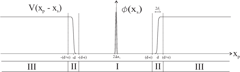
To ensure that the component in region I passes freely through the aperture, we set
| (6) |
where is a measure of the transverse spreading of the wavefunction during the interaction. We assume that the slit is thin in the -direction, and that the incident velocity of the particle is much greater than its typical transverse velocity () and that of the slit, such that the particle travels rapidly through the slit with minimal spreading. After this choice of , any small residual interaction with forces can be absorbed into the region II component.
We thus obtain an interaction of the form
| (7) | |||||
| (8) | |||||
| (9) |
where is the entangled component at the slit edge which passes through the aperture, and are components which are blocked by the slit and do not contribute to the far-field interference pattern. We leave off the slight spreading due to free evolution in the region I component as this has no effect on the transverse momentum distribution.
Under the influence of this interaction, the initial state
| (10) |
will evolve into an entangled state containing each of the terms in equations (7)-(9). We project out only the component which has successfully passed through the slit (which occurs with probability ), to obtain the final state
| (11) | |||||
| (12) |
where is a normalization constant () and is a top-hat function which projects out the wavefunction in region I, with value 1 if and 0 otherwise.
To obtain the far-field distribution, we Fourier-transform into the momentum representation (with ) to get
| (13) |
Note that the entangled component , in which forces have acted between the particle and slit, carries only a tiny fraction () of the total probability for the state, and the diffraction pattern will be largely determined by the first term. Up to small corrections due to edge effects, we therefore recover the familiar diffraction pattern in the far-field, as given by the momentum probability distribution
| (14) |
However, as the slit wavefunction is unchanged in the first term, only the small edge term can contribute to any momentum change of the slit. This is what we might expect classically, as forces are only present at the slit edge, yet the particle’s momentum distribution is largely independent of these edge forces. Instead, the form of the diffraction pattern is given by the region I contribution, in which there has been no interaction between particle and slit.
Given that the changes in particle and slit momentum arise from different terms, it is difficult to see how total momentum could be conserved in the interaction. This is not necessarily problematic, as we have projected out only part of the final state (in which the particle passes through the slit), and the total momentum distribution need only be conserved for the state as a whole. Nevertheless, it would be a surprising result.
However, with the setup given above it would be impossible to measure the momentum change of the slit. The typical momentum transferred in the scattering () will be far less than the natural uncertainty in the slit momentum () and hence, even with perfect recoil, the initial and final states of the slit will be almost identical, with overlap very close to 1. It is this feature which allows for coherent reflection of quantum particles from macroscopic objects such as mirrors[12].
For the slit recoil to have a significant effect, the momentum uncertainty of the slit must be similar in magnitude to (or less than) the momentum changes due to diffraction, as deduced by Bohr in his response to Einstein’s recoiling-slit experiment[14]. To study the momentum changes of the slit in more detail, we therefore consider a delocalized slit, with .

With the position of the slit so uncertain, it is impossible to define regions I-III for the state as a whole, but if we consider the new state of the slit as a superposition of sharp wavefunctions at different positions (fig. 3), then we can evolve each term separately as before. Dividing into narrow strips of width , and then summing over for all integer we have
| (15) |
and hence
| (16) |
Evolving each bracketed term (in which the slit has the narrow wavefunction ) as before,
| (17) | |||||
| (18) |
We neglect the small contributions from interactions close to the slit edge, and fourier-transform to the momentum representation for the particle
| (19) | |||||
| (20) |
where we have used the fourier transform relation . Finally, we reconstruct the slit wavefunction to give
| (21) |
and hence
| (22) |
The final state of the slit has the same gaussian form as the initial state, but with an average momentum of , equal and opposite to the particle momentum. We therefore obtain a simple recoil of the slit, with the momentum transfer distribution given by for any slit wavefunction. What is interesting is that the recoil derived here has nothing to do with the forces at the slit edge. The wavefunction given in equation (21) was derived entirely from region I components, in which the particle propagates freely through the centre of the slit without any interactions. In analogy with other recent works this appears to be a form of ‘interaction free’ scattering [15].
The momentum changes generated by the diffraction are a quantum phenomenon, not a direct result of forces but of entanglement in position and the intrinsic uncertainty in the slit position. Each possible slit position generates a shifted diffraction pattern, and for a given observed momentum this shift corresponds to a phase change of . As the different slit positions add coherently we obtain a slit wavefunction with an overall phase factor of and hence a momentum kick of . The role of momentum as a translational symmetry property, rather than something which is carried between particles by forces, is clearly emphasised.
This approach will be applicable whenever the particle moves rapidly through the slit, and the slit wavefunction can be broken into a large number of narrow strips which do not spread significantly during the diffraction process. It can even be applied to our original thermal slit, for which the initial velocity spread will probably be much less than that of the particle. The wavefunction could therefore be divided into small strips with increased velocities which still wouldn’t spread significantly during the interaction, and the slight momentum kick due to recoil could be explained by the above mechanism.
The apparent violation of energy conservation due to the increased transverse momenta of particle and slit can be resolved by including the -component of the wavefunction in the analysis. In addition to the transverse momentum, both longitudinal momentum and energy are conserved in the extended model (Appendix A), even though we have projected out only part of the final state.
3 Double-slit interference and which-way detection
In this section we consider the effect of which-way detection on the momentum distributions of the particle and detector in a double slit interference experiment. The setup is shown in figure 4, in which a particle with well-defined momentum is incident normally on a screen with two narrow slits. Just behind the upper slit (slit A) there is a which-way-detector, the internal state of which will change from to as the particle passes through it (as in [12]). Much further from the slits, in the far-field, there is a sensitive screen which will register the position of the particle, providing an effective measurement of its transverse momentum. As the results in the previous section can easily be extended to the double-slit itself, we focus our attention on the action of the which-way detector.

As before, we restrict our analysis to the -direction in which the slits lie, and model the particle’s propagation in the -direction by comparing initial and final states on either side of the which-way detector. The particle state just before the detector is
| (23) |
where and are wavepackets behind slits A and B respectively. We assume that is much greater than the characteristic momentum of and , such that transverse spreading is minimal while passing through the detection region.
The detector is a rigid well-localized object with a narrow wavefunction for the position of its left-hand edge (which lies in the centre of the two slits). We choose an interaction Hamiltonian of the form
| (24) |
with a constant potential within the detector and the edge effects extending over a small region as before (fig. 5). We set much lower than the kinetic energy of the particle and assume that the potential is smoothly-varying in the -direction, such that almost all particles pass through the detector without being reflected. By appropriately choosing the thickness of the detection region in the -direction, we can ensure that the internal state of the detector rotates completely from to as the wavepacket passes through it (in time ). This gives a unitary interaction of the form
| (25) |
where , and we have assumed that there is no possibility of particle reflection.

We assume that the wavepackets for the particle and detector (,,and ) are all initially separated by a distance greater than , such that they remain non-overlapping and free of edge effects throughout the interaction, with support on different regions of the -axis. This allows the detector to provide a perfect which-way measurement for the two slits, as given in equation (1). More precisely, the initial and final states are given by
| (26) | |||||
| (27) |
where we have once again neglected the slight changes due to free evolution during the detection process.
Because always generates a positive relative displacement , and a negative displacement , the interaction is not sensitive to the exact position of the detector or the forces at the detector edge and hence the spatial wavefunctions for the particle and detector remain unentangled.
In the regions of space in which the state is non-zero, the interaction potential is always constant in the -direction, with
| (28) |
Hence the particle and detector experience no transverse forces during the detection process. Yet nevertheless the particle momentum distribution is changed by the interaction, from a distribution with interference fringes to one without
| (29) |
The momentum distribution for the detector , however, remains completely unchanged, with
| (30) |
Although simple, this result is actually quite surprising; not only does the momentum of the particle change despite the absence of forces, but there is an apparent violation of total momentum conservation. Unlike the diffraction case there is no recoil of the detector, the momentum distribution of the particle simply changes on its own, without any other change to balance it.
With the particle and detector unentangled, the total momentum distribution is given by the convolution of the two individual momentum distributions . The translational symmetry of the Hamiltonian (which depends only on the relative coordinate ()) should then ensure that is conserved during the interaction. Applying this to the above case, we require that
| (31) |
In fact, this equality will hold whenever can fit into the gap between and (Appendix B), so total momentum will be conserved in the detection process described above. Note that this condition on the wavepackets is actually necessary for the detector to be able to perfectly distinguish the two particle states.
Nevertheless, this yields an interesting result: That the momentum distribution of a single particle can change in isolation without changing the total momentum distribution. This is a consequence of the convolution used to calculate the total momentum distribution, which is not a one-to-one mapping. In this case, the limited spatial support of the detector wavepacket means that some information about the particle state is discarded completely in the convolution. As the changes in particle momentum only affect this discarded region, they cause no change in the total momentum distribution.
We can also use this result to illustrate another feature of the momentum changes: That, despite the obvious differences between and , the expectation value of any finite positive integer power of the particle momentum ( for ) will be identical in the initial and final states. Using total momentum conservation,
| (32) |
where and represent expectation values in the initial and final states respectively. Since the particle and detector are unentangled (and uncorrelated), we can simplify the power expansion to get
| (33) |
Given that , this implies the inductive result that
| (34) |
As this equation is true for (, it must therefore be true by induction for all positive integer . Thus and are distributions with precisely the same moments . Those changes which do occur can be best seen by considering the modular momentum , where gives the fringe spacing in the momentum distribution. This approach is followed in more detail by Aharanov et al. [16].
4 Discussion
In both the single and double slit experiments, the momentum changes associated with the position measurement cannot be viewed as a direct result of classical forces, which vanish in the relevant regions. Instead, they depend on quantum entanglement, and the translational symmetries of the wavefunction.
In the single-slit case, we see the effect of a position measurement inside a broad incident wavefront. Here the slit provides a simple dual-valued position measurement, which tells us whether or not the particle lies inside the aperture. The uncertainty in the detector (slit) position yields a superposition of final states, in which each detector position state is entangled with a spatially-shifted particle state. In momentum-space, these spatial-shifts of the particle correspond to momentum-shifts of the detector, generating a recoil of the detector which is just as as we would classically expect - even though the scattering is ‘interaction-free’.
In the double-slit experiment, we consider the effect of a position measurement which will distinguish spatially separated parts of a wavefunction. In this case, an ideal detector can perform the measurement without becoming spatially entangled with the particle, or experiencing any recoil. Yet the momentum distribution of the particle is changed by the interaction, even though it is not subject to any transverse forces.
The fact that we can change the momentum distribution of the particle without changing the momentum distribution of the detector, and yet still conserve total momentum, is surprising. However, it emerges as a natural consequence of the convolution used to calculate the total momentum, in which some information about the momentum distributions of the individual particles is discarded.
I am grateful to Lucien Hardy, Lev Vaidman and W.Toner for useful discussions, and to EPSRC for financial support.
Appendix A
The -component of the wavefunction is important in determining when the particle passes through the aperture. Regions in which the slit is closer to the incident particle () will be diffracted sooner and thus experience a greater period of transverse spreading.
To investigate this effect, we consider the wavefunction just after the particle has passed through the slit, where it has the approximate form
| (35) |
where now includes the slit wavepacket in the z-direction, and the -component is given in terms of by equation (22). The slight transverse spreading of the wavefunction during the interaction period will introduce an additional phase factor, given by
| (36) |
where is the initial slit momentum before diffraction, is the time at which the particle passed through the slit and is the time since. The total time is constant, but the proportion of the evolution which occurs after diffraction will depend on the distance between particle and slit. Taking the particle’s speed in the -direction as and the slit as effectively static, we approximate the evolution time after diffraction by
| (37) |
which gives a phase factor of
| (38) |
Including this phase factor in the final state wavefunction will modify the -momentum of the particle to
| (39) |
with the slit receiving a momentum kick of equal magnitude in the opposite direction. Note that the momentum changes in the -direction are much smaller than those in the -direction, due to our assumptions that and . As , the change in energy is approximately given by
| (40) |
which exactly cancels the energy changes due to the increased transverse momentum of the particle and slit. Thus, at the level of these approximations, both energy and momentum are conserved in the diffraction process.
Appendix B
Proof that
| (41) |
where represents convolution and is narrower than the gap between and :
Note that spatial translations on , and on and together, of the form
| (42) | |||||
| (43) | |||||
| (44) |
have no effect on equation (41), thus without loss of generality we consider the centre of (of width ), and the centre of the gap between and (of width with ) to coincide at the origin, placing precisely in the centre of the gap.
Equation (41) is true if and only if
| (46) |
Using the Fourier-transform pair
| (47) | |||||
| (48) |
and the relations
| (49) | |||||
| (50) |
we rewrite equation (46) as
| (51) | |||||
| (52) | |||||
| (53) |
Note that the states and both lie on the same side of the origin in the region . Their convolution must therefore lie in the region . Applying the same argument to the states and we conclude that the first term in the product will be non-zero only in the region . However, the second term in the product can only be non-zero in the region . As the two functions have no common support and their product (and its Fourier-transform) will always equal zero, thus proving the validity of equation 41.
References
- [1] K.R.Popper, Die Naturwissenshaften 22, 807 (1934); K.R.Popper, Quantum Theory and the Schism in Physics (Hutchinson, London, 1983)
- [2] Y.H.Kim and Y.Shih, Found. Phys. 29, 1849 (1999) and lanl e-print quant-ph/9905039.
- [3] C.S.Unnikrishnan, Found. Phys. Lett. 13, 197 (2000)
- [4] A.J.Short, Found. Phys. Lett. 14,275 (2001)
- [5] M.Renniger, Z.Phys. 158, 417 (1960)
- [6] R.H.Dicke, Am. J. Phys. 49, 925 (1981)
- [7] R.H.Dicke, Found. Phys. 16, 107 (1986)
- [8] M.O.Scully, B.-G.Englert and H.Walther, Nature 351, 111 (1991)
- [9] P.Storey, S.Tan, M.Collett and D.Walls, Nature 367, 626 (1994)
- [10] R.P.Feynman, R.Leighton and M.Sands, The Feynman Lectures on Physics - Vol. III (Addison-Wesley, Reading, 1965)
- [11] N.Bohr in Albert Einstein: Philosopher-Scientist, edited by P.A.Schilpp (Library of living philosophers, Evanston, 1949)
- [12] L.S.Schulman, Phys. Lett. A 211, 75 (1996)
- [13] H.M.Wiseman, F.E.Harrison, M.J.Collett, S.M.Tan, D.F.Walls and R.B.Killip, Phys. Rev. A 56, 55 (1997)
- [14] A.Einstein and N.Bohr in Albert Einstein: Philosopher-Scientist, edited by P.A.Schilpp (Library of living philosophers, Evanston, 1949)
- [15] A.C.Elitzur and L.Vaidman, Found. Phys. 23, 987 (1993); L.Vaidman, lanl e-print quant-ph/0103081
- [16] Y.Aharonov, H.Pendleton, A.Petersen, Int. J. The. Phys. 3, 213 (1969)