Interference of spontaneously emitted photons
Almut Beige, Christian Schön and Jiannis Pachos
Max-Planck-Institut für Quantenoptik, 85748 Garching, Germany
e-mail: a.beige@mpq.mpg.de
Abstract: We discuss an experimental setup where two laser-driven atoms spontaneously emit photons and every photon causes a “click” at a point on a screen. By deriving the probability density for an emission into a certain direction from basic quantum mechanical principles we predict a spatial interference pattern. Similarities and differences with the classical double-slit experiment are discussed.
1 Introduction
In 1930 Werner Heisenberg wrote in [1], “It is very difficult for us to conceive the fact that the theory of photons does not conflict with the requirements of the Maxwell equations. There have been attempts to avoid the contradiction by finding solutions of the latter which represent ‘needle’ radiation (unidirectional beams), but the results could not be satisfactorily interpreted until the principles of the quantum theory had been elucidated. These show us that whenever an experiment is capable of furnishing information regarding the direction of emission of a photon, its results are precisely those which would be predicted from a solution of the Maxwell equations of the needle type (…).”

A simple quantum mechanical experiment that combines wave and particle features of emitted light is sketched in Figure 1. It shows two two-level atoms at a fixed distance that are both coupled to the same free radiation field. In addition, the atoms are excited by a resonant laser field, so that they can continuously emit photons. Each emitted photon causes a “click” at a certain point on a screen far away from the atoms. These “clicks” add up to an interference pattern with a spatial intensity distribution very similar to a classical double-slit experiment.
This setup in Figure 1 has been proposed by Scully and Drühl [2] in 1982 as a quantum eraser concerning observation and delayed choice phenomena in quantum mechanics. Their predictions were verified experimentally by Eichmann et al. in 1993 [3]. Since then the interpretation of this experiment has attracted continuous interest (see for instance Ref. [4, 5, 6, 7] and references therein). This is mainly due to its simplicity together with the fundamental quantum mechanical issues it deals with.
Recently, Schön and Beige [6] presented a quantum mechanical description of the experiment based on the assumption of environment-induced measurements. Here we first summarise the main ideas of Ref. [6] and then focus on the nature of the spatial interference of the spontaneously emitted photons. Main features of the interference pattern can also be predicted by a corresponding classical model in which the atoms are replaced by dipole sources of coherent light. Finally, similarities and differences of the two descriptions are discussed.
2 The spontaneous emission of photons
The setup shown in Figure 1 consists of two components — the quantum mechanical system including the atoms together with the free radiation field and its environment represented by the screen. The time evolution of the quantum mechanical system can be described by the Schrödinger equation. Let us denote the energy difference between the ground state and the excited state of atom at the position by whilst is the creation operator of a single photon with wave vector and polarisation . The Hamiltonian that describes the interaction between the atoms and the quantised free radiation field within the rotating wave approximation equals
| (1) |
where describes the coupling strength of the field mode and is the atomic lowering operator .
The occurrence of spontaneous “clicks” at points on the screen implies that the effect of the screen onto the quantum mechanical system can be described with the projection postulate for ideal measurements. The screen measures whether a photon has been created in the free radiation field or not [8]. If a photon is detected, then the direction [9] of its wave vector is determined [6]. The projector that describes this measurement outcome is given by
| (2) |
If no “click” is observed, then the system is projected onto a state with the free radiation field in the vacuum state . Here the atoms are continuously driven by a laser field and we assume that the screen performs rapidly repeated ideal measurements. The time between two successive measurements should not be too short, , to allow for a substantial time evolution, but also not too big so that the excitation of two-photon states in is negligible [8]. As these measurements are caused by the presence of the screen we call them environment-induced measurements.
For simplicity, let us assume that the state of the atoms at a time is known and equals while the free radiation field is in the ground state . Letting the system evolve for a short time and applying the projector (2) we find
| (3) |
where the right hand side is the unnormalised state of the system in case of a “click” in the direction away from the atoms at time . Here we assume that the dipole moment is for both atoms the same and denotes the spontaneous decay rate of a single atom in free space. Eq. (3) has been derived with the help of first order perturbation theory. For details see Section II in Ref. [6].
The norm squared of the state (3) gives the probability density for the corresponding measurement outcome,
| (4) |
The probability density for any “click” to occur can be obtained by integrating over all orientations of , leading to the product of the spontaneous decay rate and the population of the excited atomic states, namely . The “clicks” on the screen are caused by the spontaneously emitted photons. Immediately after the measurement, the excitation in the free radiation field vanishes and its state becomes again .
3 The interference pattern on the screen
Let us now specify the spatial probability density for a photon emission. If the atoms are continuously driven by a resonant laser field, their state shortly before an emission is not known. To apply the result of Eq. (4) to this situation we describe the atoms by their steady state density matrix , so becomes
| (5) | |||||
In the following we denote the Rabi frequency of the laser field with respect to atom by . Proceeding as in Ref. [6] to calculate we find that
| (6) | |||||
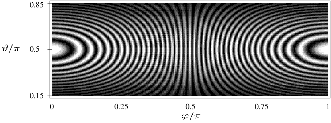
Figure 2 shows the spatial intensity distribution for the case where both laser fields are in phase and have the same intensity, i.e. . One easily recognises an interference pattern which results from the last term in Eq. (6).
To understand the origin of the interference let us assume again that the state of the atoms shortly before an emission is known and equals while the free radiation field is in the vacuum state. During the time evolution with respect to the Hamiltonian (1) each atom transfers excitation into all modes of the free radiation field. In case of a photon detection the state of the field is projected onto a photon state with the wave vector towards the direction of the “click”. To calculate the probability density for this event, one had to determine the norm of the reset state given in Eq. (3). This state is the sum of the contributions from both atoms which differ only by the phase factor . In addition, each contribution contains a different atomic state, namely or . Therefore the visibility of the interference pattern depends on the overlap of the atomic states and . If these two states are orthogonal, i.e. when the atoms are prepared in , then the probability density to find a “click” at a certain point on the screen is the sum of the probabilities of two one-atom cases. Maximum interference takes place if . This is the case when is a non-trivial superposition of the states and .
In general both atoms contribute to the spontaneous emission of a photon. Nevertheless, one could ignore this and ask from which atom the photon originated. To answer this one has to perform a measurement on the atomic state and determine whether the atoms are either in or . These two states are the reset states of the two one-atom cases where one atom emits and the state of the other one remains unchanged. Only if the reset states are orthogonal, one can find out with certainty which atom emitted the photon and the which way information is available in the experiment. In this case the interference vanishes. The more overlap the states have, the stronger becomes the visibility of the interference pattern [2, 3, 5]. For a more detailed discussion of interference criteria see also Refs. [4, 6, 7] and references therein.
4 Comparison with the classical double-slit experiment
Let us now consider a classical double-slit experiment with two dipole sources at positions and . Both dipoles have the same direction of the dipole moment and simultaneously emit electromagnetic waves with frequency . The resulting electric field at a certain point on a far away screen () is then
| (7) |
where and characterise the strength of the dipoles. The phase of the electric field produced by each source is sensitive to its position while the wave vector has in both cases, to a very good approximation, the same direction as and the amplitude . The intensity of the produced light is given by
| (8) |
The last term describes the interference pattern on the far away screen.
If we compare this spatial dependence of the interference with the spatial dependence in the quantum mechanical double-slit experiment, we see that they can in both cases be exactly the same. Nevertheless the visibility in the quantum model is in general lower than in the classical model. The reason is that population of the atomic state does not contribute to the amplitude of the interference term. In the quantum case, the more which way information is available in the experiment, the less visibility is found in the interference pattern [4]. This reduction of the visibility is a purely quantum mechanical effect.
The analogies of the quantum system with an equivalent classical one is not a surprising feature [10]. Each atom populates the free radiation field with an excitation of a certain effective frequency, , as dictated from the energy difference between the atomic levels and . In addition, when the measurement of the radiation field takes place and a photon is detected then the state of the field is projected towards a certain direction , as can be seen from Eq. (3). These two deterministic characteristics are not imposed in the initial theory as the atoms are allowed to emit with any frequency and the radiation field around them has no preference in the direction of propagation of its photon states. Nevertheless, the average along all possible photon frequencies as well as the act of detection, which projects the free radiation field onto the photon state with direction , gives the equivalence between the spontaneously emitting atoms and the classical sources.
5 Conclusions
Here we presented a quantum mechanical description of a two-atom double-slit experiment. We showed that spontaneous emission of photons can be derived from basic quantum mechanical principles by assuming environment-induced measurements on the free radiation field. By calculating the probability density for an emission into a certain direction we found spatial interference. The interference fringes appearing in the quantum case result from the spontaneously emitted photons and are not just produced by the interference of a scattered laser field. This is particularly evident in Eq. (4) where the atoms are initially prepared in an atomic state without the need for this state to be prepared by continuous laser radiation.
In general, the spatial dependence of the interference pattern and its visibility could also be described by an equivalent classical double-slit experiment. The superposition of the two amplitudes in the quantum and in the classical case produces standing waves throughout space. Their pattern is observed on the screen as seen in Figure 2.
References
- [1] W. Heisenberg, The physical principles of the quantum theory (The University of Chicago Press, Chicago 1930), Chapter V, §5.
- [2] M. O. Scully and K. Drühl, Phys. Rev. A 25, 2208 (1982).
- [3] U. Eichmann, J. C. Berquist, J. J. Bollinger, J. M. Gilligan, W. M. Itano, and D. J. Wineland, Phys. Rev. Lett. 70, 2359 (1993).
- [4] B.-G. Englert, Phys. Rev. Lett. 77, 2154 (1996).
- [5] W. M. Itano, J. C. Berquist, J. J. Bollinger, D. J. Wineland, U. Eichmann, and M. G. Raizen, Phys. Rev. A 57, 4176 (1998).
- [6] C. Schön and A. Beige, Phys. Rev. A 64, 023806 (2001).
- [7] C. Skornia, J. von Zanthier, G. S. Agarwal, E. Werner, and H. Walther, Phys. Rev. A 64, 063801 (2001).
- [8] G. C. Hegerfeldt, Phys. Rev. A 47, 449 (1993); G. C. Hegerfeldt and D.G. Sondermann, Quantum Semiclass. Opt. 8, 121 (1996).
- [9] In the following we mark normalised vectors with a hat.
- [10] For another example of equivalence between a quantum field theoretical model with a classical one see, e.g. J. Pachos, Phys. Rev. D 58, 125016 (1998).