Optimal unambiguous discrimination between subsets of non-orthogonal quantum states

According to the quantum theory of measurement, it is impossible to unambiguously discriminate between non-orthogonal quantum states with unit success probability. If, however, we settle for less and don’t require that we succeed every time, then unambiguous discrimination becomes possible. This procedure uses a non-unitary operation that maps the non-orthogonal states onto orthogonal ones, and these can then be discriminated without error using a standard von Neuman measurement. Although such an operation will always have a certain probability of failure, we can always tell whether or not the desired transformation has succeeded. This allows us to achieve unambiguous discrimination. When the attempt fails, we obtain an inconclusive answer. The optimal strategy for accomplishing this is the one that minimizes the average probability of failure.

The problem of unambiguously distinguishing between two non-orthogonal states was first considered by Ivanovic ivanovic, and then subsequently by Dieks dieks and Peres peres2. These authors found the optimal solution when the two states are being selected from an ensemble in which they are equally likely. The optimal solution for the situation in which the states have different weights was found by Jaeger and Shimony jaeger. We proposed an optical implementation of the optimal procedure along with a more compact rederivation of the general results and also showed that the method is useful in other areas of quantum information processing sun1 such as, for example, entanglement enhancement chefles4. State discrimination measurements have been performed in laboratory, first by Huttner, et. al. huttner and, more recently, by Clarke, et al. clarke. Both used the polarization states of photons to represent qubits. The case of three states was examined by Peres and Terno peres3. It was subsequently extended to the general problem of discriminating among $N$ states. Chefles chefles2 found that $N$ non-orthogonal states can be probabilistically discriminated without error if and only if they are linearly independent. Chefles and Barnett chefles3 solved the case in which the probability of the procedure succeeding is the same for each of the states. Duan and Guo duan considered general unitary transformations and measurements on a Hilbert space containing the states to be distinguished and an ancilla, which would allow one to discriminate among $N$ states, and derived matrix inequalities which must be satisfied for the desired transformations to exist. In our previous paper sun2, we presented the necessary conditions for optimal unambiguous discrimination and used them to derive a method for implementing the optimal solution. For the case of three states, we presented optical networks that accomplish this. One can also consider what happens if the discrimination is not completely unambiguous, i. e. if it is possible for errors to occur, and this was done by Chefles and Barnett chefles1. For an overview of the state-of-the-art on state discrimination see the excellent recent review article by Chefles chefrev.

In these works discrimination among all of the states was considered. In the present paper, we consider a variant of that problem. Instead of discriminating among all states, we ask what happens if we just want to discriminate between subsets of them. A motivation to consider this variant comes from its application to comparing strings of qubits in order to find out if they are identical or not which is certainly one of the basic tasks in quantum information processing. In particular, if there are three non-orthogonal states, $\{|\psi_{1}\rangle,|\psi_{2}\rangle,|\psi_{3}\rangle\}$, we wish to find the optimal strategy to unambiguously distinguish $|\psi_{1}\rangle$ from the set $\{|\psi_{2}\rangle,|\psi_{3}\rangle\}$. We refer to this problem as unambiguous quantum state filtering. In this context we should note that recently an analytical solution has been found to the following closely related problem. Instead of unambiguously distinguishing between two complementary subsets of an arbitary number $N$ of non-orthogonal quantum states, occupying a two-dimensional Hilbert space, errors are allowed but the probability of erroneously assigning the state to one of the substes is minimized HB. The term “quantum state filtering” has been introduced there for the case when one of the subsets contains one state and the other contains all of the remaining $N-1$ states. Here, we shall present the analytical solution for the case of the other possible discrimnation strategy, namely that of unambiguous quantum state filtering.

The paper is divided into six sections. In Section II, based on simple but rigorous arguments, we present the optimal analytical solution to the problem. In Section III, we compare these optimal failure probabilities for two different procedures: discrimination between $|\psi_{1}\rangle$ and $\{|\psi_{2}\rangle,|\psi_{3}\rangle\}$ and discrimination among all three states. We find that the failure probability for the first procedure is smaller than that for the second. In Section IV, we propose a possible experimental implementation using the method proposed in our previous paper sun2, which uses a single-photon representation of the quantum states and an optical multiport together with photon detection at the output ports to implement the procedure. A brief discussion and conclusions are given in Section V. Finally, in the Appendix, we present an alternative derivation, based on the method of Lagrange multipliers, to obtain the results of Section II. The method closely parallels the techniques used for unambiguous discrimination between all states.

Suppose we are given a quantum system prepared in the state $|\psi\rangle$, which is guaranteed to be a member of the set of three non-orthogonal states $\left\{|\psi_{1}\rangle,|\psi_{2}\rangle,|\psi_{3}\rangle\right\}$, but we do not know which one. We want to find a procedure which will tell us that $|\psi\rangle$ was prepared in $|\psi_{1}\rangle$, or will tell us that $|\psi\rangle$ was prepared in one of $\left\{|\psi_{2}\rangle,|\psi_{3}\rangle\right\}$. That is, the procedure can distinguish $|\psi_{1}\rangle$ from $\left\{|\psi_{2}\rangle,|\psi_{3}\rangle\right\}$. We also want this procedure to be error-free, i. e. the procedure may fail to give us any information about the state, and if it fails, it must let us know that it has, but if it succeeds, it should never give us a wrong answer. We shall refer to such a procedure as quantum state filtering without error. We find that, in contrast to the unambiguous state discrimination problem, this will be possible even if $|\psi_{1}\rangle$ is not linearly independent from the set $\{|\psi_{2}\rangle,|\psi_{3}\rangle\}$.

If the states are not orthogonal then, according to the quantum theory of measurement, they cannot be discriminated perfectly. In other words, if we are given $|\psi_{i}\rangle$, we will have some probability $p_{i}$ to determine what it is successfully and, correspondingly, some failure probability, $q_{i}=1-p_{i}$, to obtain an inconclusive answer. If we denote by $\eta_{i}$ the a priori probability that the system was prepared in the state $|\psi_{i}\rangle$, the average probabilities of success and of failure to distinguish the states $|\psi_{i}\rangle$ are

respectively. Our objective is to find the set of $\left\{p_{i}\right\}$ that maximizes the probability of success, $P$.

The procedure we shall use is a “generalized measurement”, which can be described as follows. Let $\mathcal{K}$ denote a total Hilbert space, which is the direct sum of two subspaces, $\mathcal{K}=\mathcal{H}\oplus\mathcal{A}$. The space $\mathcal{H}$ is a three-dimensional space that contains the vectors $|\psi_{i}\rangle$, and $\mathcal{A}$ is an auxiliary space. The input state of the system is one of the vectors $|\psi_{i}\rangle$, which is now a vector in the subspace $\mathcal{H}$ of the total space $\mathcal{K}$, so that

A unitary transformation, $U$, which acts in the entire space $\mathcal{K}$ is now applied to the input vector, resulting in the state $|\psi_{i}^{\mathcal{K}}\rangle_{out}$, which is given by

where, in our case, $|\psi_{1}^{\prime}\rangle$ can always be unambiguously distinguished from the set $\{|\psi_{2}^{\prime}\rangle,|\psi_{3}^{\prime}\rangle\}$. Then a measurement is performed on $|\psi_{i}^{\mathcal{K}}\rangle_{out}$ that projects $|\psi_{i}^{\mathcal{K}}\rangle_{out}$ either onto $|\psi_{i}^{\prime}\rangle$ or $|\phi_{i}\rangle$ (by construction, they are in orthogonal subspaces). If it projects $|\psi_{i}^{\mathcal{K}}\rangle_{out}$ onto $|\psi_{i}^{\prime}\rangle$, the procedure succeeds, because $|\psi_{1}^{\prime}\rangle$ can always be distinguished from $\{|\psi_{2}^{\prime}\rangle,|\psi_{3}^{\prime}\rangle\}$. The probability to get this outcome, if the input state is $|\psi_{i}\rangle$, is

If the measurement projects $|\psi_{i}^{\mathcal{K}}\rangle_{out}$ onto $|\phi_{i}\rangle$, the procedure fails. The probability of this outcome is

The nature of the problem we are trying to solve imposes a number of requirements on the output vectors. The condition that $|\psi_{1}^{\prime}\rangle$ be distinguishable from $|\psi_{2}^{\prime}\rangle$ and $|\psi_{3}^{\prime}\rangle$ requires that

These lead to conditions on the failure vectors, $|\phi_{i}\rangle$. Taking the scalar product between $|\psi^{\mathcal{K}}_{1}\rangle_{out}$ and the other two output states and using Eq. (6) and the fact that $U$ is unitary leads to the conditions

Our objective is to find the optimal $|\psi_{i}^{\prime}\rangle$ and $|\phi_{i}\rangle$ which satisfy Eqs. (4)– (II) and also give the maximum success probability $P$.

Let us now consider the failure vectors. If they were linearly independent, we could apply a state discrimination procedure to them chefles2. That means that if our original procedure fails, and we end up in the failure space, $\mathcal{A}$, then we still have some chance of determining what our input state was. This clearly implies that our original procedure, which led to the vectors $|\psi^{\prime}\rangle$, was not optimal, because that process followed by another on the failure vectors would lead to a higher probability of distinguishing $|\psi_{1}\rangle$ from $|\psi_{2}\rangle$ and $|\psi_{3}\rangle$. Therefore, the optimal procedure should lead to failure vectors to which we cannot successfully apply a state discrimination procedure, implying that they are linearly dependent. In fact, we will now prove that for optimal discrimination they must be collinear, by demonstrating that the contrary leads to contradiction. To this end, we assume that we have achieved optimal unambiguous discrimination of $|\psi_{1}\rangle$ from $|\psi_{2}\rangle$ and $|\psi_{3}\rangle$ but the failure vectors are not collinear. Then at least one of the two failure vectors, $|\phi_{2}\rangle$, $|\phi_{3}\rangle$, will have a component in the direction that is perpendicular to $|\phi_{1}\rangle$. We can set up a detector projecting onto this direction and a positive outcome of the measurement (a click of the detector) will tell us that our input state was not $|\psi_{1}\rangle$ but one of the other two states. Thus, contrary to our assumption that our procedure has been optimal, further distinction is possible. Hence, the failure vectors must be collinear for optimal discrimination.

We shall now explore the consequences of this conclusion. Since $|\phi_{i}\rangle$ ($i=1,\ldots,n)$ are collinear, the failure space, $\mathcal{A}$, is one dimensional. If $|u\rangle$ is the basis vector spanning this Hilbert space we can write the failure vectors as $|\phi_{i}\rangle=\sqrt{q_{i}}e^{\chi_{i}}|u\rangle$. Substituting this representation of the failure vectors into Eq. (II), we find that

These two conditions are a consequence of unitarity and imply that only one of the three failure probabilities can be chosen independently. If we chose $q_{1}$ as the independent one we can express the other two as $q_{2}=|\langle\psi_{1}|\psi_{2}\rangle|^{2}/q_{1}$ and $q_{3}=|\langle\psi_{1}|\psi_{3}\rangle|^{2}/q_{1}$. If we introduce the notation $O_{ij}=\langle\psi_{i}|\psi_{j}\rangle$ then, with the help of these two equations, the average failure probability can be written explicitly as

If we further introduce the notation $A=\eta_{2}|O_{12}|^{2}+\eta_{3}|O_{13}|^{2}$ for the frequently occuring average overlap then, from the condition

we find the optimal value of $q_{1}$ to be

This value, however, cannot always be realized. For it to be true, there must be a unitary transformation, from Eq. (3), that takes $|\psi_{j}\rangle$ to $|\psi_{j}\rangle_{out}$ which, together with the one-dimensionality of the failure space yields

Here we have that $\langle\psi_{j}^{\prime}|u\rangle=0$, $\langle\psi_{1}^{\prime}|\psi_{j}^{\prime}\rangle=0$ for $j=2,3$, and the phase factors are fixed by the requirement (cf. Eq. (II)) that

for $j=2,3$. These equations imply that

This set of equations can only be true if the matrix $M$, where

is positive semidefinite, as discussed in detail in Ref. sun2.

Using again $O_{jk}=\langle\psi_{j}|\psi_{k}\rangle$, $M$ can be expressed as

Clearly, this matrix will be positive semidefinite if $0\leq q_{1}\leq 1$, and if the $2\times 2$ submatrix is also positive semidefinite. This will be true if both the trace and determinant of the submatrix are greater than or equal to zero. Positivity requires that the diagonal matrix elements of the submatrix be non-negative, so that it must be true that $q_{1}\geq|O_{12}|$ and $q_{1}\geq|O_{13}|$ . Without loss of generality, we can assume that $|O_{12}|\geq|O_{13}|$ by simply arranging the states in set $2$ in the order of decreasing overlaps with $|\psi_{1}\rangle$. Doing so and imposing the condition that $q_{1}\geq|O_{12}|$ guarantees that the condition $q_{1}\geq|O_{13}|$ is also satisfied, and together they imply that the trace is greater than or equal to zero.

The condition that the determinant be non-negative gives us a lower bound on $q_{1}$,

We want to interpret this inequality, in particular, we want to find what the right-hand side is equal to. In order to do so, we shall find the projection operator, $P_{23}$, that projects onto the subspace spanned by $\psi_{2}$ and $\psi_{3}$. One of the basis vectors in this subspace can be chosen to be $|\psi_{2}\rangle$ and, using the Gram-Schmidt orthogonalization method, the other is defined as the (normalized) orthogonal component of $|\psi_{3}\rangle$,

This leads to

Let us represent the input state, $|\psi_{1}\rangle$, as $|\psi_{1}\rangle=|\psi^{\perp}_{1}\rangle+|\psi^{\parallel}_{1}\rangle$, where $|\psi^{\perp}_{1}\rangle=(1-P_{23})|\psi_{1}\rangle$ is the component of the input vector that is perpendicular to the subspace spanned by $\psi_{2}$ and $\psi_{3}$ and $|\psi^{\parallel}_{1}\rangle=P_{23}|\psi_{1}\rangle$ is the component in that subspace. Then, using Eqs. (18) and (19), the explicit expression for the parallel component is given by

Calculating the norm of this expression yields

which is identical to the right-hand side of Eq. (17).

Thus, Eq. (17) tells us that the failure probability, $q_{1}$, has a lower bound which is given by the weight of $|\psi_{1}\rangle$ in the other subspace, $\|P_{23}\psi_{1}\|^{2}=\langle\psi_{1}|P_{23}|\psi_{1}\rangle=\langle\psi^{\parallel}_{1}|\psi^{\parallel}_{1}\rangle$, a result that is intuitively obvious. Clearly, this expression is larger than (or at most equal to) $|O_{12}|^{2}$. This implies that, because $q_{2}=|O_{12}|^{2}/q_{1}$, we have

and similarly for $q_{3}$.

We can then distinguish three different regimes of the parameters. If the r.h.s. of Eq. (11) is greater than $1$ then $q_{1}=1$, if it is less than $\langle\psi^{\parallel}_{1}|\psi^{\parallel}_{1}\rangle$ then $q_{1}=\langle\psi^{\parallel}_{1}|\psi^{\parallel}_{1}\rangle$, and in the intermediate range the optimum given by Eq. (11) is realized. This can be summarized as follows.

(i) If $\eta_{1}|\langle\psi^{\parallel}_{1}|\psi^{\parallel}_{1}\rangle|^{2}\leq A\leq\eta_{1}$, then

yielding the average failure probability

(ii) If $A\geq\eta_{1}$, then

yielding the average failure probability

(iii) If $A\leq\eta_{1}|\langle\psi^{\parallel}_{1}|\psi^{\parallel}_{1}\rangle|^{2}$, then

yielding the average failure probability

Equations (II)–(28) summarize our main results. In the intermediate range of the average overlap, $A$, the optimal failure probability, Eq. (24), is achieved by a generalized measurement or POVM. Outside this region, for very large average overlap, $A\geq\eta_{1}$, or very small average overlap, $A\leq\eta_{1}|\langle\psi^{\parallel}_{1}|\psi^{\parallel}_{1}\rangle|^{2}$, the optimal failure probabilities, Eqs. (26) and (28), are realized by standard von Neumann measurements. For very large $A$ the optimal von Neumann measurement consists of projections onto $|\psi_{1}\rangle$ and two orthogonal directions whose directionality needs not be specified further. A click along $|\psi_{1}\rangle$ corresponds to failure because it can have its origin in any of the two subsets and a click in the orthogonal directions uniquely assigns the input state to the set $\{|\psi_{2}\rangle,|\psi_{3}\rangle\}$. For very small $A$ the optimal von Neumann measurement consists of projections onto $|\psi^{\parallel}_{1}\rangle$ and two orthogonal directions that are uniquely determined by the requirement that they correspond to two mutually exclusive alternatives. One of them is onto $|\psi^{\perp}_{1}\rangle$ and the other onto the remaining orthogonal direction in the subspace of $\{|\psi_{2}\rangle,|\psi_{3}\rangle\}$. A click along $|\psi^{\parallel}_{1}\rangle$ corresponds to failure because it can originate from any of the input states while a click in any of the alternative directions unambiguously assigns the input to one or the other of the two mutually exclusive subsets. It is interesting to observe that the failure space is one dimensional for each of the three different optimal measurements in the three different regions. At the boundaries of their respective regions of validity, the optimal measurements transform into one another continuously. Furthermore, each of the two von Neumann expressions can be written as the arithmetic mean of two terms and the POVM result as the geometric mean of the same two terms. Therefore, in its range of validity the POVM performs better than any von Neumann measurement.

In closing this Section we want to point out an interesting feature of the solution. The results hold true even when there is no perpendicular component of the first input state, $|\psi^{\perp}_{1}\rangle=0$, i.e. it lies entirely in the Hilbert space spanned by the other two vectors or, in other words, the two sets are linearly dependent. In this case the two von Neumann measurements coincide and the range of validity of the POVM solution shrinks to zero. A click in the detector along the first input vector corresponds to failure - it might originate from either of the two subsets - and a click in the detector along the single direction orthogonal to it unambiguously identifies the set of the other two vectors.

An alternative derivation of the above results, that is based on the method of Langrange multipliers, is given in the Appendix.

In this section we want to compare the average probability of failure $Q$ of the filtering problem to that of distinguishing all three states. Let $Q^{\prime}$ denote the average probability of failure for distinguishing all the states $\{|\psi_{1}\rangle,|\psi_{2}\rangle,|\psi_{3}\rangle\}$. We can see immediately, that the probability of failure to distinguish $|\psi_{1}\rangle$ from $\{|\psi_{2}\rangle,|\psi_{3}\rangle\}$, $Q$, should be no larger than $Q^{\prime}$. For the latter problem, the necessary condition for achieving optimal discrimination is

When comparing this equation to Eq. (A), we see that, instead of a given constant $O_{23}$ that appears in Eq. (29), there are the variables $r$ and $\theta$ in Eq. (A). These variables are chosen to minimize the average probability of failure $Q$. Therefore, $Q$ should be no larger than $Q^{\prime}$, $Q\leq Q^{\prime}$.

To illustrate this point, we use a simple symmetric case, where all of the overlaps between the states are real and equal,

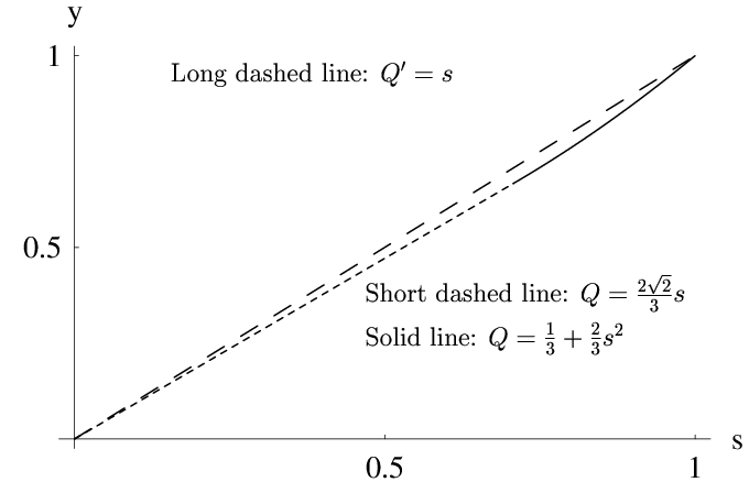
with $0<s<1$. We shall also assume that the a priori probabilities are equal for all the examples in this paper. From previous work we know that in this case, the optimal values of the failure probabilities when we wish to distinguish among all of the states $\{|\psi_{1}\rangle,|\psi_{2}\rangle,|\psi_{3}\rangle\}$ are $q_{i}=s$, which implies that $Q^{\prime}=s$ sun2.

For the problem of distinguishing $|\psi_{1}\rangle$ from $\{|\psi_{2}\rangle,|\psi_{3}\rangle\}$, from the results of Eqs. (II) and (II), we have (i) if $0<s\leq\frac{\sqrt{2}}{2}$, then

So the average probability of failure $Q$ is less than $Q^{\prime}=s$. (ii) if $\frac{\sqrt{2}}{2}<s<1$, then

These solutions are illustrated and compared to $Q^{\prime}$ in Figure 1. Note that in both cases we have that $Q<s=Q^{\prime}$.

Now we shall compare filtering to the problem of distinguishing two states $\{|\psi_{1}\rangle,|\psi_{2}\rangle\}$, when all the a priori probabilities are equal. If we denote by $Q^{\prime\prime}$ the average probability of failure when distinguishing between the two states $\{|\psi_{1}\rangle$ and $|\psi_{2}\rangle\}$, we know that $Q^{\prime\prime}=|O_{12}|$ (Refs. ivanovic–jaeger). For the case we are considering, $|O_{12}|=|O_{13}|=s$, and we see that $Q<Q^{\prime\prime}$.

A second example is more illuminating. The overlaps are now given by

where, for simplicity, $s_{1}$ and $s_{2}$ are real, $0<s_{1},s_{2}<1$, and

The probabilities of failure for discriminating $|\psi_{1}\rangle$ from $\{|\psi_{2}\rangle,|\psi_{3}\rangle\}$ are

and the average failure probability is

The optimal probabilities of failure for discriminating among all three states $\{|\psi_{1}\rangle,|\psi_{2}\rangle,|\psi_{3}\rangle\}$ are given by sun2

$Q$ can be compared to $Q^{\prime}$ by examining the ratio

From the above equation, we see that when $s_{1}$ is much smaller than $s_{2}$, $Q$ is much smaller than $Q^{\prime}$. For example, when $s_{1}=\frac{\sqrt{2}}{5}$, $s_{2}=\frac{4}{5}$, $Q/Q^{\prime}=0.47$.

Now we shall present a scheme for a possible experimental realization of the optimal discrimination between $|\psi_{1}\rangle$ and $\{|\psi_{2}\rangle,|\psi_{3}\rangle\}$. The method is similar to one we proposed in a previous publication sun2. We shall use single photon states to represent the input and output states, and an optical eight-port together with photon detectors placed at the output ports to realize the unitary transformation and subsequent measurements.

Our states will be a single photon split among several modes. Each mode will serve as an input to an optical eight-port. Recall that the dimension of the total Hilbert space is four, so we shall require four modes, and the input states $|\psi_{i}\rangle$ will be represented by single photon states as

where $\sum_{j=1}^{4}|d_{ij}|^{2}=1$, and $\hat{a}_{j}^{\dagger}$ is the creation operator for the $j$th mode. We shall require $d_{i4}=0$ for $i=1,2,3$, that is, the initial single photon state is sent to the first three input ports, and the vacuum into the fourth input port. The first three modes correspond to the space, $\mathcal{H}$, containing the states to be distinguished and the fourth mode to the failure space, $\mathcal{A}$.

In general, an optical $2N$-port is a lossless linear device with $N$ input ports and $N$ output ports. Its action on the input states can be described by a unitary operator, $U_{2N}$, and physically it consists of an arrangement of beam splitters, phase shifters, and mirrors. Since the dimension of the input and output states is four, here we shall use an eight-port (see Figure 2).

To design the desired eight-port, we first calculate the optimal value of $q_{i}$. Then from Eq. (5) and the fact that our failure space is one-dimensional, the vectors $|\phi_{i}\rangle$ are given by

where the state $|1^{\mathcal{A}}\rangle$ denotes one photon state in the failure space, which is just one photon in mode $4$. Once the vectors $|\phi_{i}\rangle$ are determined, the inner products $\langle\psi_{i}^{\prime}|\psi_{j}^{\prime}\rangle$ $(i,j=1,2,3)$ are given by

We then have to find vectors $|\psi_{i}^{\prime}\rangle$ that satisfy this equation. The answer is not unique, and one way of proceeding is the following. If we define the hermitian matrix $L$ to be

then we note from Eq. (II) that $L_{12}=L_{13}=0$. This implies that the simplest choice for $|\psi_{1}^{\prime}\rangle$ is a vector with only one nonzero component. Then the vectors $|\psi_{2}^{\prime}\rangle$ and $|\psi_{3}^{\prime}\rangle$ will have nonzero components in only their other two places. The obvious choice is

In this column vector, the first entry is the amplitude of the photon to be in mode $1$, the second is the amplitude to be in mode $2$, etc. Mode $4$ corresponds to the failure space, $\mathcal{A}$. The vectors $|\psi_{2}^{\prime}\rangle$ and $|\psi_{3}^{\prime}\rangle$ will have nonzero components in only their second and third places, and if their overlap is real, we can choose

where

This simple choice works for the last example in this section (see Eq. (IV), below). For the first, somewhat more general, example we are forced to choose the second component of $|\psi_{1}^{\prime}\rangle$ to be nonzero and then the first and third components of the other two success vectors are different from zero. They can be obtained by simply interchanging the first and second components in the above expressions of the vectors $|\psi_{i}^{\prime}\rangle$ (see Eq. (IV), below).

Once we have the input and output vectors, the unitary transformation, $U$, which maps the input states onto the output states then can be chosen, and this, as shown by Eq. (41), gives the explicit form of $M(4)$. Furthermore, $M(4)$ can be factorized as a product of two-dimensional $U(2)$ transformationssun2; reck, and any $U(2)$ transformations can be implemented by a lossless beam splitter and a phase shifter with appropriate parameters. A beam splitter with a phase shifter at one output port transforms the input operators into output operators as

where $a_{1}$, $a_{2}$ are the annihilation operators of modes 1 and 2 respectively, $\omega$ describes the reflectivity and transmittance of the beam splitter, and $\phi$ describes the effect of the phase shifter (in the factorization method given by M. Reck et al. reck, the phase shifters described by $\phi$ should be placed at the input ports). Therefore, we can use appropriate beam splitters, phase shifters and a mirror to construct the desired eight-port.

Finally, photon detection is performed at the four output ports. We can design the total transformation in such a way that if the photon is detected at the first output port, we claim with certainty that the initial state was $|\psi_{1}\rangle$, if the photon is detected at the second or the third output port, we claim with certainty that the initial state was either $|\psi_{2}\rangle$ or $|\psi_{3}\rangle$, but we do not know which of these two states it was. If the photon is detected at the fourth output port, we obtain no information about the input state.

We shall now consider two examples. The first is more general than the second, but the second has the advantage that it is simple and the eight-port that it requires consists of only two $50-50$ beam splitters. In the first example, all of the input vectors have the same overlap, which is given by $s$, and we shall consider the case $0<s\leq 1/\sqrt{2}$. The optimal failure probabilities for this case are given in Eq. (III). For the input vectors we shall take

The output vectors, $|\psi_{i}\rangle_{out}=|\psi^{\prime}_{i}\rangle+|\phi_{i}\rangle$, can be computed by the method outlined above. Doing so gives us

Our next step is to determine the transformation, $U$, that describes the eight-port, or, more specifically, the matrix $M(4)$ that describes its action in the one-photon subspace. It must satisfy $|\psi_{i}\rangle_{out}=U|\psi\rangle_{in}$, and, in addition, it must map the vector that is orthogonal to all three input vectors, onto the vector that is orthogonal to all three output vectors,

where

These equations determine M(4) and it is given by $M(4)=$

This matrix can be expressed as the product of three matrixes each of which corresponds to a beam splitter. In particular, we have that

where the matrix $T_{p,q}$ represents the action of a beam splitter that mixes only modes $p$ and $q$. The $4\times 4$ matrix for $T_{p,q}$ can be obtained from that of a $4\times 4$ identity matrix, $I$, by replacing the matrix elements $I_{pp}$ and $I_{qq}$ by the transmissivity of the beam splitter, $t$, replacing $I_{pq}$ by the reflectivity, $r$, and replacing $I_{qp}$ by $-r$. The transmissivities and reflectivities for beam splitters in Eq. (82) are

This constitutes a complete description of the optical network that optimally discriminates between $|\psi_{1}\rangle_{in}$ and $\{|\psi_{2}\rangle_{in},|\psi_{3}\rangle_{in}\}$, where these input states are given in Eq. (IV), and it is shown schematically in Figure 3.

An especially simple network will suffice for our second example. The input vectors are

These input states have the property that

The optimal failure probabilities are found to be $q_{1}=2/3$ and $q_{2}=q_{3}=1/3$. Using Eqs. (34) and (35) this gives

for the minimum average failure probability of this kind of generalized measurement. This is to be compared to $5/9$, the average failure probability of a von Neuman type projective measurement.

The output vectors, $|\psi_{i}\rangle_{out}=|\psi^{\prime}_{i}\rangle+|\phi_{i}\rangle$, can again be computed by the method outlined previously. Doing so gives us

References

- (1) I. D. Ivanovic, Phys. Lett. A 123, 257 (1987).
- (2) D. Dieks, Phys. Lett. A 126, 303 (1988).
- (3) A. Peres, Phys. Lett. A 128, 19 (1988).
- (4) G. Jaeger and A. Shimony, Phys. Lett. A 197, 83 (1995).
- (5) J. Bergou, M. Hillery, and Y. Sun, J. Mod. Opt. 47, 487 (2000).
- (6) A. Chefles and S. M. Barnett, Phys. Lett. A 236, 177 (1997).
- (7) B. Huttner, A. Muller, J. D. Gautier, H. Zbinden, and N. Gisin, Phys. Rev. A 54, 3783 (1996).
- (8) R. B. M. Clarke, A. Chefles, S. M. Barnett, and E. Riis, Phys. Rev. A 63, 040305 (R) (2001).
- (9) A. Peres and D. Terno, J. Phys. A 31, 7105 (1998).
- (10) A. Chefles, Phys. Lett. A239, 339 (1998).
- (11) A. Chefles and S. M. Barnett, Phys. Lett. A250, 223 (1998).
- (12) L-M. Duan and G-C. Guo, Phys. Lett. A261, 25 (1999).
- (13) Y. Sun, M. Hillery and J. A. Bergou, Phys. Rev. A 64, 022311 (2001); and J. Bergou, M. Hillery and Y. Sun, Fortschr. Phys. 49, 915 (2001), where a preliminary version of the current problem was first formulated.
- (14) A. Chefles and S. M. Barnett, J. Mod. Opt. 45, 1295 (1998).
- (15) A. Chefles, Contemp. Phys. 41, 401 (2000).
- (16) U. Herzog and J. Bergou, Phys. Rev. A65, 050305(R) (2002).
- (17) M. Reck, A. Zeilinger, H. J. Bernstein and P. Bertani, Phys. Rev. Lett. 73, 58 (1994).
- (18) The case is presently being investigated by ourselves and independently by S. M. Barnett, A. Chefles, and I. Jex.