跳到论文正文
W Papers独立论文阅读器 arXiv:quant-ph/0111050 论文正文 计算阅读时间 · 0%
引用这篇论文根据当前论文元数据生成,正式投稿前建议核对。


License: Assumed arXiv.org perpetual non-exclusive license
arXiv:quant-ph/0111050v1 [quant-ph] 08 Nov 2001

Generalised boundary conditions for the Aharonov-Bohm effect combined with a homogeneous magnetic field

P. Exner    P. Šťovíček    P. Vytřas
Abstract

The most general admissible boundary conditions are derived for an idealised Aharonov-Bohm flux intersecting the plane at the origin on the background of a homogeneous magnetic field. A standard technique based on self-adjoint extensions yields a four-parameter family of boundary conditions; other two parameters of the model are the Aharonov-Bohm flux and the homogeneous magnetic field. The generalised boundary conditions may be regarded as a combination of the Aharonov-Bohm effect with a point interaction. Spectral properties of the derived Hamiltonians are studied in detail.

1Nuclear Physics Institute, Academy of Sciences, 250 68 Řež near Prague, Czech Republic
2Department of Mathematics, Faculty of Nuclear Science, Czech Technical University, Trojanova 13, 120 00 Prague, Czech Republic
3Doppler Institute, Czech Technical University, Břehová 7, 115 19 Prague, Czech Republic

1 Introduction

The purpose of this paper is to determine the most general admissible boundary conditions for the Aharonov-Bohm (AB) effect in the plane on the background of a homogeneous magnetic field, and also to investigate the basic properties of Hamiltonians obtained this way. The history of the effect goes four decades back and starts from the observation of Aharonov and Bohm [1] that the behavior of a charged quantum particle is influenced by a magnetic flux even if the field is zero in the region where the particle is localized. A particularly elegant treatment is possible in case of an idealized setup in which the AB flux is concentrated along a line perpendicularly intersecting the plane, conventionally at the origin [2].

The boundary conditions of the last mentioned paper are not the most general ones; the full family of such conditions giving the AB effect in the plane was derived in [7], and simultaneously also in [8]. These generalised boundary conditions may be interpreted as a combination of the AB effect with a point interaction supported, too, at the origin, although this is just one possible point of view. In any case they can be described and investigated by the technique of self-adjoint extensions which is in principle the same one as that used in the paper [6] in which two-dimensional point interactions were introduced.

A natural question is what happens if such a system is placed into a background homogeneous magnetic field. This problem attracted some attention recently, even with a controversy: the papers [3, 4, 5] consider the “pure” AB effect in this setting for the Pauli operator, i.e. a spin 1/21/2 particle. The last named property leads to specific behavior related to the Aharonov-Casher effect, which we will not discuss here.

Our aim here is different: we are going to consider a spinless particle with a point flux and a homogeneous background, and ask about the most general class of boundary conditions analogous to those of [7, 8]. The basic difference between the situations without and with a homogeneous magnetic field is that in the former case the spectrum is absolutely continuous and equal to the positive half-line possibly augmented with at most two negative eigenvalues (depending on the choice of boundary conditions) while in the latter case the spectrum is pure point and the point flux and interaction gives rise to eigenvalues in each gap between neighboring Landau levels. Our goal is to discuss these spectral properties in detail.

2 Formulation of the problem, preliminaries

We consider the symmetric operator

L=−(∇−A(∇))2, Dom(L)=C0∞(ℝ2∖{0}),L=-(\nabla-A(\nabla))^{2},\textrm{ }\mathop{\mathrm{Dom}}(L)=C_{0}^{\infty}(\mathbb{R}^{2}\setminus\{0\}),

where the vector potential AA is a sum of two parts, A=Ahmf+AABA=A_{\mathrm{hmf}}+A_{\mathrm{AB}}, with the part AhmfA_{\mathrm{hmf}} corresponding to the homogeneous magnetic field in the circular gauge,

Ahmf=−ı​B2​(−x2​d​x1+x1​d​x2),A_{\mathrm{hmf}}=-\frac{\imath B}{2}(-x_{2}dx_{1}+x_{1}dx_{2}),

and with the part AABA_{\mathrm{AB}} corresponding to the idealised AB effect,

AAB=ı​Φ2​π​r2(−x2dx1+x1dx2), r2=x1 2+x2 2.A_{\mathrm{AB}}=\frac{\imath\Phi}{2\pi r^{2}}(-x_{2}dx_{1}+x_{1}dx_{2}),\textrm{ }r^{2}=x_{1}^{\,2}+x_{2}^{\,2}.

Without loss of generality we may assume that B>0B>0. Further, we rescale the Aharonov-Bohm flux,

α=−Φ2​π,\alpha=-\frac{\Phi}{2\pi},

to have a variable which expresses the number of flux quanta and, as usual, we make use of the gauge symmetry allowing us to assume that α∈]0,1[\alpha\in\,]0,1[\,. Hence the case Φ∈2​π​ℤ\Phi\in 2\pi\mathbb{Z} is excluded since it is gauge equivalent to the vanishing AB flux. Our goal is to describe all the self-adjoint extensions of LL as well as to investigate their basic properties.

It is straightforward to determine the adjoint operator L∗L^{\ast},

ψ∈Dom(L∗)​\displaystyle\psi\in\mathop{\mathrm{Dom}}(L^{\ast})\textrm{ } ⟺\displaystyle\Longleftrightarrow ψ∈L2​(ℝ2,d2​x)∩Hloc2,2​(ℝ2∖{0})\displaystyle\psi\in L^{2}(\mathbb{R}^{2},\mathrm{d}^{2}x)\cap H^{2,2}_{\mathrm{loc}}(\mathbb{R}^{2}\setminus\{0\})
and ​(∇−A⁡(∇))2​ψ∈L2​(ℝ2,d2​x).\displaystyle\textrm{and }(\nabla-A(\nabla))^{2}\psi\in L^{2}(\mathbb{R}^{2},\mathrm{d}^{2}x).

Next we can employ the rotational symmetry when using the polar coordinates (r,θ)(r,\theta) and decomposing the Hilbert space into the orthogonal sum of the eigenspaces of the angular momentum,

L2​(ℝ2,d2​x)=∑⊕m∈ℤ⊕​L2​(ℝ+,r​d​r)⊗ℂ​eı​m​θ.L^{2}(\mathbb{R}^{2},\mathrm{d}^{2}x)=\sideset{}{{}^{\oplus}}{\sum}_{m\in\mathbb{Z}}L^{2}(\mathbb{R}_{+},r\,\mathrm{d}r)\otimes\mathbb{C}\,e^{\imath m\theta}. (1)

In the polar coordinates the operator LL (and correspondingly L∗L^{\ast}) takes the form

L=−1r∂rr∂r+1r2(−ı∂θ+α+B​r22)2.L=-\frac{1}{r}\,\partial_{r}r\partial_{r}+\frac{1}{r^{2}}\left(-\imath\partial_{\theta}+\alpha+\frac{Br^{2}}{2}\right)^{2}.

The operator L∗L^{\ast} commutes on Dom(L∗)\mathop{\mathrm{Dom}}(L^{\ast}) with the projectors PmP_{m} onto the eigenspaces of the angular momentum,

Pm​ψ​(r,θ)=12​π​∫02​πψ⁡(r,θ′)​eı​m​(θ−θ′)​d​θ′,P_{m}\psi(r,\theta)=\frac{1}{2\pi}\int_{0}^{2\pi}\psi(r,\theta^{\prime})\,e^{\imath m(\theta-\theta^{\prime})}\,\mathrm{d}\theta^{\prime},

and therefore L∗L^{\ast} decomposes in correspondence with the orthogonal sum (1),

L∗=∑⊕m∈ℤ⊕​(L∗)m.L^{\ast}=\sideset{}{{}^{\oplus}}{\sum}_{m\in\mathbb{Z}}(L^{\ast})_{m}. (2)

Thus we can reduce the problem and work in the sectors RanPm\mathop{\mathrm{Ran}}P_{m}, m∈ℤm\in\mathbb{Z}. For a given spectral parameter λ∈ℂ\lambda\in\mathbb{C} we choose two independent solutions (except of particular values of λ\lambda) of the differential equation

(−1r∂rr∂r+1r2(m+α+B​r22)2)g(r)=λg(r),\left(-\frac{1}{r}\,\partial_{r}r\partial_{r}+\frac{1}{r^{2}}\left(m+\alpha+\frac{Br^{2}}{2}\right)^{2}\right)g(r)=\lambda\,g(r), (3)

namely

gm1​(λ,r)\displaystyle g^{1}_{m}(\lambda;r) =r|m+α|​F​(β⁡(m,λ),γ⁡(m),B​r22)​exp⁡(−B​r24),\displaystyle=r^{|m+\alpha|}\,F\left(\beta(m,\lambda),\gamma(m),\frac{Br^{2}}{2}\right)\exp\left(-\frac{Br^{2}}{4}\right), (4)
gm2​(λ,r)\displaystyle g^{2}_{m}(\lambda;r) =r|m+α|​G​(β⁡(m,λ),γ⁡(m),B​r22)​exp⁡(−B​r24),\displaystyle=r^{|m+\alpha|}\,G\left(\beta(m,\lambda),\gamma(m),\frac{Br^{2}}{2}\right)\exp\left(-\frac{Br^{2}}{4}\right),

where

β⁡(m,λ)\displaystyle\beta(m,\lambda) =12​(1+m+α+|m+α|−λB),\displaystyle=\frac{1}{2}\left(1+m+\alpha+|m+\alpha|-\frac{\lambda}{B}\right), (5)
γ⁡(m)\displaystyle\gamma(m) =1+|m+α|.\displaystyle=1+|m+\alpha|\,.

Here FF and GG are confluent hypergeometric functions [9, Chp. 13],

F⁡(β,γ,z)=∑n=0∞(β)n​zn(γ)n​n!,F(\beta,\gamma,z)=\sum^{\infty}_{n=0}\frac{(\beta)_{n}\,z^{n}}{(\gamma)_{n}\,n!}\,,

and

G⁡(β,γ,z)=Γ⁡(1−γ)Γ⁡(β−γ+1)​F​(β,γ,z)+Γ⁡(γ−1)Γ⁡(β)​z1−γ​F​(β−γ+1,2−γ,z).G(\beta,\gamma,z)=\frac{\Gamma(1-\gamma)}{\Gamma(\beta-\gamma+1)}\,F(\beta,\gamma,z)+\frac{\Gamma(\gamma-1)}{\Gamma(\beta)}\,z^{1-\gamma}F(\beta-\gamma+1,2-\gamma,z). (6)

Notice that F⁡(β,γ,z)F(\beta,\gamma,z) and G⁡(β,γ,z)G(\beta,\gamma,z) are linearly dependent if and only if β∈−ℤ+\beta\in-\mathbb{Z}_{+}. Moreover, F⁡(β,γ,z)F(\beta,\gamma,z) is an entire function, particularly, it is regular at the origin while G⁡(β,γ,z)G(\beta,\gamma,z) has a singularity there provided γ>1\gamma>1 and β∉−ℤ+\beta\notin-\mathbb{Z}_{+}, and in that case it holds true that

limz→0+zγ−1​G​(β,γ,z)=Γ⁡(γ−1)Γ⁡(β).\lim_{z\to 0_{+}}z^{\gamma-1}G(\beta,\gamma,z)=\frac{\Gamma(\gamma-1)}{\Gamma(\beta)}\,.

Thus in the case when 1<γ<21<\gamma<2 we have the asymptotic behaviour, as z→0+z\to 0_{+},

G⁡(β,γ,z)=Γ⁡(γ−1)Γ⁡(β)​z1−γ+Γ⁡(1−γ)Γ⁡(β−γ+1)+O⁡(z2−γ).G(\beta,\gamma,z)=\frac{\Gamma(\gamma-1)}{\Gamma(\beta)}\,z^{1-\gamma}+\frac{\Gamma(1-\gamma)}{\Gamma(\beta-\gamma+1)}+O(z^{2-\gamma}). (7)

We shall also need some information about the asymptotic behaviour at infinity. When z→+∞z\to+\infty it holds true that

F⁡(β,γ,z)=Γ⁡(γ)Γ⁡(γ−β)​(−z)−β​(1+O⁡(z−1))+Γ⁡(γ)Γ⁡(β)​ez​zβ−γ​(1+O⁡(z−1))F(\beta,\gamma,z)=\frac{\Gamma(\gamma)}{\Gamma(\gamma-\beta)}\,(-z)^{-\beta}\left(1+O\left(z^{-1}\right)\right)+\frac{\Gamma(\gamma)}{\Gamma(\beta)}\,e^{z}z^{\beta-\gamma}\left(1+O\left(z^{-1}\right)\right) (8)

and

G⁡(β,γ,z)=z−β​(1+O⁡(z−1)).G(\beta,\gamma,z)=z^{-\beta}\left(1+O\left(z^{-1}\right)\right).

3 The standard Aharonov-Bohm Hamiltonian

With the above preliminaries it is straightforward to solve the spectral problem for the standard AB Hamiltonian as we mentioned in the introduction. This means to solve the eigenvalue problem

L∗​ψ=λ​ψL^{\ast}\psi=\lambda\psi

with the boundary condition

limr→0+ψ⁡(r,θ)=0.\lim_{r\to 0_{+}}\psi(r,\theta)=0. (9)

By virtue of the decomposition (2) the problem is reduced to the countable set of equations

(L∗)mf=λf, m∈ℤ,(L^{\ast})_{m}f=\lambda f,\textrm{ }m\in\mathbb{Z},

and hence to the differential equations (3).

The solution gm2​(λ,r)g^{2}_{m}(\lambda;r) of (3) is ruled out because it contradicts the condition (9) and the solution gm1​(λ,r)g^{1}_{m}(\lambda;r) belongs to L2​(ℝ+,r​d​r)L^{2}(\mathbb{R}_{+},r\,\mathrm{d}r) if and only if β⁡(m,λ)=−n\beta(m,\lambda)=-n, with n∈ℤ+n\in\mathbb{Z}_{+}. Since it holds

F(−n,1+σ,z)=n!​Γ​(σ+1)Γ⁡(n+σ+1)Lnσ(z), n∈ℤ+,F(-n,1+\sigma,z)=\frac{n!\,\Gamma(\sigma+1)}{\Gamma(n+\sigma+1)}\,L_{n}^{\sigma}(z),\textrm{ }n\in\mathbb{Z}_{+},

we get a countable set of eigenvalues,

λm,n=B(m+α+|m+α|+2n+1), m∈ℤ, n∈ℤ+,\lambda_{m,n}=B\,(m+\alpha+|m+\alpha|+2n+1),\textrm{ }m\in\mathbb{Z},\textrm{ }n\in\mathbb{Z}_{+},

with the corresponding eigenfunctions

fm,n​(r,θ)=Cm,n​r|m+α|​Ln|m+α|​(B​r22)​exp⁡(−B​r24)​eı​m​θf_{m,n}(r,\theta)=C_{m,n}\,r^{|m+\alpha|}\,L_{n}^{|m+\alpha|}\left(\frac{Br^{2}}{2}\right)\,\exp\left(-\frac{Br^{2}}{4}\right)\,e^{\imath m\theta}

where

Cm,n=(B2)12​(|m+α|+1)​(n!π​Γ​(n+|m+α|+1))1/2C_{m,n}=\left(\frac{B}{2}\right)^{\frac{1}{2}(|m+\alpha|+1)}\left(\frac{n!}{\pi\,\Gamma(n+|m+\alpha|+1)}\right)^{1/2}

are the normalisation constants.

As it is well known if we fix m∈ℤm\in\mathbb{Z} then the functions {fm,n​(r,θ)}n=0∞\{f_{m,n}(r,\theta)\}^{\infty}_{n=0} form an orthonormal basis in L2​(ℝ+,r​d​r)⊗ℂ​eı​m​θL^{2}(\mathbb{R}_{+},r\,\mathrm{d}r)\otimes\mathbb{C}\,e^{\imath m\theta} and so the complete set of eigenfunctions {fm,n(r,θ)}m∈ℤ, n∈ℤ+\{f_{m,n}(r,\theta)\}_{m\in\mathbb{Z}\,,\textrm{ }n\in\mathbb{Z}_{+}} is an orthonormal basis in L2​(ℝ+,r​d​r)⊗L2​([ 0,2​π],d​θ)L^{2}(\mathbb{R}_{+},r\,\mathrm{d}r)\otimes L^{2}([\,0,2\pi\,],\mathrm{d}\theta). Since all the eigenvalues λm,n\lambda_{m,n} are real we get this way a well defined self-adjoint operator which is an extension of LL. We conventionally call it the standard AB Hamiltonian and denote it by HA​BH^{AB}. Thus the spectrum of HA​BH^{AB} is pure point and can be written as a union of two parts,

σ(HA​B)=σp​p(HA​B)={B(2k+1); k∈ℤ+}∪{B(2α+2k+1); k∈ℤ+}.\sigma(H^{AB})=\sigma_{pp}(H^{AB})=\{B(2k+1);\textrm{ }k\in\mathbb{Z}_{+}\}\cup\{B(2\alpha+2k+1);\textrm{ }k\in\mathbb{Z}_{+}\}.

Notice that the eigenvalues belonging to the first part are nothing but the Landau levels. All the eigenvalues B⁡(2​k+1)B(2k+1) have infinite multiplicities while the multiplicity of the eigenvalue B⁡(2​α+2​k+1)B(2\alpha+2k+1) is finite and equals k+1k+1.

A final short remark concerning the Hamiltonian HA​BH^{AB} is devoted to the Green function. Naturally, the Green function is expressible as an infinite series

GA​B​(z,r1,θ1,r2,θ2)=12​π​∑m=−∞∞GmA​B​(z,r1,r2)​eı​m​(θ1−θ2)G^{AB}(z;r_{1},\theta_{1},r_{2},\theta_{2})=\frac{1}{2\pi}\sum_{m=-\infty}^{\infty}G_{m}^{AB}(z;r_{1},r_{2})\,e^{\imath m(\theta_{1}-\theta_{2})}

where

GmA​B​(z,r1,r2)\displaystyle G_{m}^{AB}(z;r_{1},r_{2}) =\displaystyle= 2​(B2)|m+α|+1​(r1​r2)|m+α|​exp⁡(−14​B​(r1 2+r2 2))\displaystyle 2\left(\frac{B}{2}\right)^{|m+\alpha|+1}(r_{1}r_{2})^{|m+\alpha|}\exp\left(-\frac{1}{4}\,B(r_{1}^{\ 2}+r_{2}^{\ 2})\right)
×∑n=0∞n!Γ⁡(n+|m+α|+1)\displaystyle\times\sum_{n=0}^{\infty}\,\frac{n!}{\Gamma(n+|m+\alpha|+1)}
×Ln|m+α|​(12​B​r1 2)​Ln|m+α|​(12​B​r2 2)B⁡(m+α+|m+α|+2​n+1)−z.\displaystyle\quad\times\frac{L_{n}^{|m+\alpha|}(\frac{1}{2}Br_{1}^{\ 2})\,L_{n}^{|m+\alpha|}(\frac{1}{2}Br_{2}^{\ 2})}{B(m+\alpha+|m+\alpha|+2n+1)-z}\,.

The radial parts can be rewritten with the aid of the standard construction of the Green function for ordinary differential operators of second order,

GmA​B​(z,r1,r2)\displaystyle G_{m}^{AB}(z;r_{1},r_{2}) =\displaystyle= (B2)|m+α|+1​(r1​r2)|m+α|​exp⁡(−14​B​(r1 2+r2 2))\displaystyle\left(\frac{B}{2}\right)^{|m+\alpha|+1}(r_{1}r_{2})^{|m+\alpha|}\exp\left(-\frac{1}{4}\,B(r_{1}^{\ 2}+r_{2}^{\ 2})\right)
×Γ⁡(−w⁡(m,z))Γ⁡(|m+α|+1)​F​(−w⁡(m,z),|m+α|+1,r<)\displaystyle\times\,\frac{\Gamma\big(-w(m,z)\big)}{\Gamma(|m+\alpha|+1)}\,F(-w(m,z),|m+\alpha|+1,r_{<})
×G⁡(−w⁡(m,z),|m+α|+1,r>)\displaystyle\times\,G(-w(m,z),|m+\alpha|+1,r_{>})

where

w⁡(m,z)=z2​B−12​(m+α+|m+α|+1)w(m,z)=\frac{z}{2B}-\frac{1}{2}(m+\alpha+|m+\alpha|+1)

and r<=min⁡(r1,r2)r_{<}=\min(r_{1},r_{2}), r>=max⁡(r1,r2)r_{>}=\max(r_{1},r_{2}). This amounts to the identity

∑n=0∞n!Γ⁡(n+σ+1)​Lnσ​(y1)​Lnσ​(y2)n−w\displaystyle\sum_{n=0}^{\infty}\,\frac{n!}{\Gamma(n+\sigma+1)}\,\frac{L_{n}^{\sigma}(y_{1})\,L_{n}^{\sigma}(y_{2})}{n-w}
=Γ⁡(−w)Γ⁡(σ+1)​F​(−w,σ+1,y<)​G​(−w,σ+1,y>).\displaystyle\qquad=\,\frac{\Gamma(-w)}{\Gamma(\sigma+1)}\,F(-w,\sigma+1,y_{<})\,G(-w,\sigma+1,y_{>}).

We do not expect that a simpler form for the Green function could be derived since the Hamiltonian HA​BH^{AB} enjoys only the rotational symmetry.

4 Self-adjoint extensions of LL

Recalling what has been summarised in Section 2 it is easy to determine the deficiency indices. The solution gm1​(±ı,r)g^{1}_{m}(\pm\imath;r) diverges exponentially at infinity (cf. (8)) while gm2​(±ı,r)g^{2}_{m}(\pm\imath;r) behaves well at infinity but has a singularity at the origin of the order r−|m+α|r^{-|m+\alpha|}. Thus gm2​(±ı,r)∈L2​(ℝ+,r​d​r)g^{2}_{m}(\pm\imath;r)\in L^{2}(\mathbb{R}_{+},r\,\mathrm{d}r) if and only if m=−1m=-1 or m=0m=0. This means that the deficiency indices are (2,2)(2,2). For a basis in the deficiency subspaces 𝒩±ı{\cal N}_{\pm\imath} we can choose

{fm,±(r,θ)=12​πNmgm2(±ı;r)eı​m​θ; m=−1,0}.\{f_{m,\pm}(r,\theta)=\frac{1}{\sqrt{2\pi}}\,N_{m}\,g^{2}_{m}(\pm\imath;r)\,e^{\imath m\theta};\textrm{ }m=-1,0\}.

Thus

f−1,±​(r,θ)\displaystyle f_{-1,\pm}(r,\theta) =\displaystyle= 12​π​N−1​r1−α​G​(12∓ı2​B,2−α,B​r22)​exp⁡(−B​r24)​e−ı​θ,\displaystyle\frac{1}{\sqrt{2\pi}}\,N_{-1}\,r^{1-\alpha}\,G\left(\frac{1}{2}\mp\frac{\imath}{2B},2-\alpha,\frac{Br^{2}}{2}\right)\,\exp\left(-\frac{Br^{2}}{4}\right)\,e^{-\imath\theta},
f0,±​(r,θ)\displaystyle f_{0,\pm}(r,\theta) =\displaystyle= 12​π​N0​rα​G​(12+α∓ı2​B,1+α,B​r22)​exp⁡(−B​r24),\displaystyle\frac{1}{\sqrt{2\pi}}\,N_{0}\,r^{\alpha}\,G\left(\frac{1}{2}+\alpha\mp\frac{\imath}{2B},1+\alpha,\frac{Br^{2}}{2}\right)\,\exp\left(-\frac{Br^{2}}{4}\right),

where N−1N_{-1} and N0N_{0} are normalisation constants making the basis orthonormal.

We shall need the explicit values of N−1N_{-1} and N0N_{0}. Using the relation

Wυ,τ(z)=zτ+12e−z/2G(12−υ+τ,2τ+1,z)W_{\upsilon,\tau}(z)=z^{\tau+\frac{1}{2}}e^{-z/2}\,G\left(\frac{1}{2}-\upsilon+\tau,2\tau+1,z\right)

where WW is the Whittaker function we get

Nm−2\displaystyle N_{m}^{\ -2} =\displaystyle= ∫0∞|gm2​(±ı,r)|2​r​𝑑r\displaystyle\int^{\infty}_{0}|g^{2}_{m}(\pm\imath;r)|^{2}\,r\mathrm{d}r
=\displaystyle= 12​(2B)|m+α|+1​∫0∞x−1​Wϱ,σ​(x)​Wϱ¯,σ​(x)​𝑑x\displaystyle\frac{1}{2}\left(\frac{2}{B}\right)^{|m+\alpha|+1}\int_{0}^{\infty}x^{-1}W_{\varrho,\sigma}(x)\,W_{\bar{\varrho},\sigma}(x)\,\mathrm{d}x

where

ϱ=12(−m−α+ıB), σ=12|m+α|.\varrho=\frac{1}{2}\left(-m-\alpha+\frac{\imath}{B}\right),\textrm{ }\sigma=\frac{1}{2}\,|m+\alpha|.

Combining the identities [10, 2.19.24.6]

∫0∞x−1​Wϱ,σ​(x)​Wμ,σ​(x)​𝑑x=πsin⁡(2​π​σ)\displaystyle\int^{\infty}_{0}x^{-1}W_{\varrho,\sigma}(x)\,W_{\mu,\sigma}(x)\,\mathrm{d}x=\frac{\pi}{\sin(2\pi\sigma)}
×(−1Γ⁡(12−σ−μ)​Γ​(32+σ−ϱ)​F12​(12+σ−μ,1,32+σ−ϱ,1)CLOSE\displaystyle\qquad\times\,\Biggl(-\frac{1}{\Gamma\left(\frac{1}{2}-\sigma-\mu\right)\,\Gamma\left(\frac{3}{2}+\sigma-\varrho\right)}\,{}_{2}{F_{1}}\biggl(\frac{1}{2}+\sigma-\mu,1;\frac{3}{2}+\sigma-\varrho;1\biggr)
OPEN+1Γ⁡(12+σ−μ)​Γ​(32−σ−ϱ)​F12​(12−σ−μ,1,32−σ−ϱ,1))\displaystyle\qquad\phantom{\times\,\Biggl(}+\frac{1}{\Gamma\left(\frac{1}{2}+\sigma-\mu\right)\,\Gamma\left(\frac{3}{2}-\sigma-\varrho\right)}\,{}_{2}{F_{1}}\biggl(\frac{1}{2}-\sigma-\mu,1;\frac{3}{2}-\sigma-\varrho;1\biggr)\Biggr)

and

F12​(a,b,c,z)=\displaystyle{}_{2}{F_{1}}(a,b;c;z)\,=
Γ⁡(c)​Γ​(c−a−b)Γ⁡(c−a)​Γ​(c−b)​F12​(a,b,a+b−c+1,1−z)\displaystyle\qquad\frac{\Gamma(c)\,\Gamma(c-a-b)}{\Gamma(c-a)\,\Gamma(c-b)}\,{}_{2}{F_{1}}(a,b;a+b-c+1;1-z)
+Γ⁡(c)​Γ​(a+b−c)Γ⁡(a)​Γ​(b)​(1−z)c−a−b​F12​(c−a,c−b,c−a−b+1,1−z)\displaystyle\qquad+\,\frac{\Gamma(c)\,\Gamma(a+b-c)}{\Gamma(a)\,\Gamma(b)}\,(1-z)^{c-a-b}{}_{2}{F_{1}}(c-a,c-b;c-a-b+1;1-z)

we arrive at the relation

∫0∞x−1​Wϱ,σ​(x)​Wμ,σ​(x)​𝑑x=πsin⁡(2​π​σ)​(μ−ϱ)\displaystyle\int^{\infty}_{0}x^{-1}W_{\varrho,\sigma}(x)\,W_{\mu,\sigma}(x)\,\mathrm{d}x=\frac{\pi}{\sin(2\pi\sigma)(\mu-\varrho)}
×(−1Γ⁡(12−μ−σ)​Γ​(12−ϱ+σ)+1Γ⁡(12−μ+σ)​Γ​(12−ϱ−σ)).\displaystyle\qquad\times\left(-\frac{1}{\Gamma\left(\frac{1}{2}-\mu-\sigma\right)\,\Gamma\left(\frac{1}{2}-\varrho+\sigma\right)}+\frac{1}{\Gamma\left(\frac{1}{2}-\mu+\sigma\right)\,\Gamma\left(\frac{1}{2}-\varrho-\sigma\right)}\right).

Finally we get

N−1\displaystyle N_{-1} =\displaystyle= (B2)12​(1−α)sin⁡(π​α)2​π(Im1Γ⁡(−12+α+ı2​B)​Γ​(12−ı2​B))−1/2,\displaystyle\left(\frac{B}{2}\right)^{\frac{1}{2}(1-\alpha)}\sqrt{\frac{\sin(\pi\alpha)}{2\pi}}\,\left(\Imp\frac{1}{\Gamma\left(-\frac{1}{2}+\alpha+\frac{\imath}{2B}\right)\,\Gamma\left(\frac{1}{2}-\frac{\imath}{2B}\right)}\right)^{-1/2},
N0\displaystyle N_{0} =\displaystyle= (B2)12​αsin⁡(π​α)2​π(Im1Γ⁡(12+ı2​B)​Γ​(12+α−ı2​B))−1/2.\displaystyle\left(\frac{B}{2}\right)^{\frac{1}{2}\alpha}\sqrt{\frac{\sin(\pi\alpha)}{2\pi}}\,\left(\Imp\frac{1}{\Gamma\left(\frac{1}{2}+\frac{\imath}{2B}\right)\,\Gamma\left(\frac{1}{2}+\alpha-\frac{\imath}{2B}\right)}\right)^{-1/2}.

Let us have a look at the asymptotic behaviour at the origin of the basis functions in the deficiency subspaces 𝒩±ı{\cal N}_{\pm\imath}. By (4) and (7) we have

g−12​(±ı,r)\displaystyle g^{2}_{-1}(\pm\imath;r) =a−1,±​r−1+α+b−1,±​r1−α+O⁡(r1+α),\displaystyle=a_{-1,\pm}\,r^{-1+\alpha}+b_{-1,\pm}\,r^{1-\alpha}+O(r^{1+\alpha}), (10)
g02​(±ı,r)\displaystyle g^{2}_{0}(\pm\imath;r) =a0,±​r−α+b0,±​rα+O⁡(r2−α),\displaystyle=a_{0,\pm}\,r^{-\alpha}+b_{0,\pm}\,r^{\alpha}+O(r^{2-\alpha}),

where

a−1,±=Γ⁡(1−α)Γ⁡(12∓ı2​B)​(B2)−1+α\displaystyle a_{-1,\pm}=\frac{\Gamma(1-\alpha)}{\Gamma\left(\frac{1}{2}\mp\frac{\imath}{2B}\right)}\,\left(\frac{B}{2}\right)^{-1+\alpha} ,\displaystyle,\textrm{ } b−1,±=Γ⁡(−1+α)Γ⁡(−12+α∓ı2​B),\displaystyle b_{-1,\pm}=\frac{\Gamma(-1+\alpha)}{\Gamma\left(-\frac{1}{2}+\alpha\mp\frac{\imath}{2B}\right)}\,,
a0,±=Γ⁡(α)Γ⁡(12+α∓ı2​B)​(B2)−α\displaystyle a_{0,\pm}=\frac{\Gamma(\alpha)}{\Gamma\left(\frac{1}{2}+\alpha\mp\frac{\imath}{2B}\right)}\,\left(\frac{B}{2}\right)^{-\alpha} ,\displaystyle,\textrm{ } b0,±=Γ⁡(−α)Γ⁡(12∓ı2​B).\displaystyle b_{0,\pm}=\frac{\Gamma(-\alpha)}{\Gamma\left(\frac{1}{2}\mp\frac{\imath}{2B}\right)}\,.

The coefficients am,±a_{m,\pm}, bm,±b_{m,\pm} are related to the normalisation constants NmN_{m} for it holds true that

detM−1=−ı1−α(N−1)−2, detM0=−ıα(N0)−2.\det M_{-1}=-\frac{\imath}{1-\alpha}\,(N_{-1})^{-2},\textrm{ }\det M_{0}=-\frac{\imath}{\alpha}\,(N_{0})^{-2}. (11)

where

Mm=(am,+bm,+am,−bm,−).M_{m}=\left(\begin{array}[]{cc}a_{m,+}&b_{m,+}\\ a_{m,-}&b_{m,-}\end{array}\right).

Particularly, we shall need the fact that the matrices M−1M_{-1} and M0M_{0} are regular.

Let us now describe the closure of the operator LL. In virtue of the decomposition (2) we have

L¯=∑⊕m∈ℤ⊕​L¯m\bar{L}=\sideset{}{{}^{\oplus}}{\sum}_{m\in\mathbb{Z}}\bar{L}_{m}

where L¯m=(L∗)m∗\bar{L}_{m}=(L^{\ast})_{m}^{\,\ast}. As it is well known, ψ∈Dom(L∗)\psi\in\mathop{\mathrm{Dom}}(L^{\ast}) belongs to Dom(L¯)\mathop{\mathrm{Dom}}(\bar{L}) if and only if ⟨ψ,L∗​φ⟩=⟨L∗​ψ,φ⟩\left\langle\psi,L^{\ast}\varphi\right\rangle=\left\langle L^{\ast}\psi,\varphi\right\rangle for all φ∈𝒩ı+𝒩−ı\varphi\in{\cal N}_{\imath}+{\cal N}_{-\imath}. Thus (L∗)m=L¯m(L^{\ast})_{m}=\bar{L}_{m} for m≠{−1,0}m\neq\{-1,0\}, and if m∈{−1,0}m\in\{-1,0\} then φ⁡(r)​eı​m​θ∈Dom((L∗)m)\varphi(r)\,e^{\imath m\theta}\in\mathop{\mathrm{Dom}}((L^{\ast})_{m}) belongs to Dom(L¯m)\mathop{\mathrm{Dom}}(\bar{L}_{m}) if and only if

limr→0+r​W​(φ⁡(r)¯,gm2​(±ı,r))=0\lim_{r\to 0_{+}}r\,W(\overline{\varphi(r)},g^{2}_{m}(\pm\imath,r))=0

where W⁡(f,g)=(∂rf)​g−f​∂rgW(f,g)=(\partial_{r}f)g-f\,\partial_{r}g is the Wronskian. Using the asymptotic behaviour (10) and the regularity of the matrix MmM_{m} we arrive at two conditions

limr→0+(−|m+α|​r−|m+α|​φ​(r)−r−|m+α|+1​∂rφ⁡(r))=0,\displaystyle\lim_{r\to 0_{+}}(-|m+\alpha|\,r^{-|m+\alpha|}\varphi(r)-r^{-|m+\alpha|+1}\partial_{r}\varphi(r))=0,
limr→0+(|m+α|​r|m+α|​φ​(r)−r|m+α|+1​∂rφ⁡(r))=0,\displaystyle\lim_{r\to 0_{+}}(|m+\alpha|\,r^{|m+\alpha|}\varphi(r)-r^{|m+\alpha|+1}\partial_{r}\varphi(r))=0,

which can be rewritten in the equivalent form,

limr→0+r−2​|m+α|+1∂r(r|m+α|φ(r))=0, limr→0+r|m+α|φ(r)=0.\lim_{r\to 0_{+}}r^{-2|m+\alpha|+1}\partial_{r}(r^{|m+\alpha|}\varphi(r))=0,\textrm{ }\lim_{r\to 0_{+}}r^{|m+\alpha|}\varphi(r)=0.

But since

r−|m+α|​|φ⁡(r)|≤12​|m+α|​supx∈]0,r[|x−2​|m+α|+1​∂x(x|m+α|​φ​(x))|r^{-|m+\alpha|}|\varphi(r)|\leq\frac{1}{2|m+\alpha|}\,\sup_{x\in\,]0,r[}|x^{-2|m+\alpha|+1}\partial_{x}(x^{|m+\alpha|}\varphi(x))|

we finally get a sufficient and necessary condition for φ⁡(r)​eı​m​θ∈Dom((L∗)m)\varphi(r)\,e^{\imath m\theta}\in\mathop{\mathrm{Dom}}((L^{\ast})_{m}) to belong to Dom(L¯)\mathop{\mathrm{Dom}}(\bar{L}), namely

limr→0+r−1+α​φ​(r)=0​ and ​limr→0+rα​φ′​(r)=0\displaystyle\lim_{r\to 0_{+}}r^{-1+\alpha}\varphi(r)=0\text{ and }\lim_{r\to 0_{+}}r^{\alpha}\varphi^{\prime}(r)=0 if\displaystyle\quad\text{if } m=−1,\displaystyle m=-1, (12)
limr→0+r−α​φ​(r)=0​ and ​limr→0+r−α+1​φ′​(r)=0\displaystyle\lim_{r\to 0_{+}}r^{-\alpha}\varphi(r)=0\text{ and }\lim_{r\to 0_{+}}r^{-\alpha+1}\varphi^{\prime}(r)=0 if\displaystyle\quad\text{if } m=0.\displaystyle m=0.

This shows that if ψ∈Dom(L∗)=Dom(L¯)+𝒩ı+𝒩−ı\psi\in\mathop{\mathrm{Dom}}(L^{\ast})=\mathop{\mathrm{Dom}}(\bar{L})+{\cal N}_{\imath}+{\cal N}_{-\imath} then

ψ⁡(r,θ)\displaystyle\psi(r,\theta) =\displaystyle= (Φ11​(ψ)​r−1+α+Φ21​(ψ)​r1−α)​e−ı​θ+Φ12​(ψ)​r−α+Φ22​(ψ)​rα\displaystyle\left(\Phi^{1}_{1}(\psi)r^{-1+\alpha}+\Phi^{1}_{2}(\psi)r^{1-\alpha}\right)e^{-\imath\theta}+\Phi^{2}_{1}(\psi)r^{-\alpha}+\Phi^{2}_{2}(\psi)r^{\alpha}
+ a regular part.\displaystyle+\textrm{ a regular part}.

Let us formally introduce the functionals Φjk\Phi_{j}^{k} on Dom(L∗)\mathop{\mathrm{Dom}}(L^{\ast}),

Φ1−1​(ψ)\displaystyle\Phi^{-1}_{1}(\psi) =\displaystyle= limr→0+r1−α​12​π​∫02​πψ⁡(r,θ)​eı​θ​𝑑θ,\displaystyle\lim_{r\to 0_{+}}r^{1-\alpha}\frac{1}{2\pi}\int^{2\pi}_{0}\psi(r,\theta)\,e^{\imath\theta}\mathrm{d}\theta,
Φ2−1​(ψ)\displaystyle\Phi^{-1}_{2}(\psi) =\displaystyle= limr→0+r−1+α​(12​π​∫02​πψ⁡(r,θ)​eı​θ​𝑑θ−Φ11​(ψ)​r−1+α),\displaystyle\lim_{r\to 0_{+}}r^{-1+\alpha}\left(\frac{1}{2\pi}\int^{2\pi}_{0}\psi(r,\theta)\,e^{\imath\theta}\mathrm{d}\theta-\Phi^{1}_{1}(\psi)\,r^{-1+\alpha}\right),
Φ10​(ψ)\displaystyle\Phi^{0}_{1}(\psi) =\displaystyle= limr→0+rα​12​π​∫02​πψ⁡(r,θ)​𝑑θ,\displaystyle\lim_{r\to 0_{+}}r^{\alpha}\frac{1}{2\pi}\int^{2\pi}_{0}\psi(r,\theta)\mathrm{d}\theta,
Φ20​(ψ)\displaystyle\Phi^{0}_{2}(\psi) =\displaystyle= limr→0+r−α​(12​π​∫02​πψ⁡(r,θ)​𝑑θ−Φ12​(ψ)​r−α).\displaystyle\lim_{r\to 0_{+}}r^{-\alpha}\left(\frac{1}{2\pi}\int^{2\pi}_{0}\psi(r,\theta)\mathrm{d}\theta-\Phi^{2}_{1}(\psi)\,r^{-\alpha}\right).

Notice that the upper index refers to the sector of angular momentum while the lower index refers to the order of the singularity. If ψ∈Dom(L¯)\psi\in\mathop{\mathrm{Dom}}(\bar{L}) then according to (12) it actually holds Φjk​(ψ)=0\Phi^{k}_{j}(\psi)=0 for j=1,2j=1,2, k=−1,0k=-1,0. On the other hand, if ψ∈𝒩ı+𝒩−ı\psi\in{\cal N}_{\imath}+{\cal N}_{-\imath} and Φjk​(ψ)=0\Phi^{k}_{j}(\psi)=0 for all indices j=1,2j=1,2, k=−1,0k=-1,0, then ψ=0\psi=0 (this is again guaranteed by the regularity of the matrices M−1M_{-1} and M0M_{0}).

Let us introduce some more notation. It is convenient to arrange the functionals Φjk\Phi^{k}_{j} into column vectors as follows,

Φj(ψ)=(Φj−1​(ψ)Φj0​(ψ)), j=1,2.\Phi_{j}(\psi)=\left(\begin{array}[]{c}\Phi^{-1}_{j}(\psi)\\ \Phi^{0}_{j}(\psi)\end{array}\right),\textrm{ }j=1,2.

Further, applying the functionals to the basis functions in 𝒩ı+𝒩−ı{\cal N}_{\imath}+{\cal N}_{-\imath} we obtain four 2×22\times 2 diagonal matrices. More precisely, set

(Φj,±)k​ℓ=2​πΦjk−2(fℓ−2,±), j,k,ℓ=1,2.\left(\Phi_{j,\pm}\right)_{k\ell}=\sqrt{2\pi}\,\Phi_{j}^{k-2}(f_{\ell-2,\pm}),\textrm{ }j,k,\ell=1,2.

Then

Φ1,±=(N−1​a−1,±00N0​a0,±), Φ2,±=(N−1​b−1,±00N0​b0,±).\Phi_{1,\pm}=\left(\begin{array}[]{cc}N_{-1}a_{-1,\pm}&0\\ 0&N_{0}\,a_{0,\pm}\end{array}\right),\textrm{ }\Phi_{2,\pm}=\left(\begin{array}[]{cc}N_{-1}b_{-1,\pm}&0\\ 0&N_{0}\,b_{0,\pm}\end{array}\right).

Now it is straightforward to give a formal definition of a self-adjoint extension HUH^{U} of the symmetric operator LL determined by a unitary operator U:𝒩ı→𝒩−ıU:{\cal N}_{\imath}\to{\cal N}_{-\imath}. We identify UU with a unitary 2×22\times 2 matrix via the choice of the orthonormal bases {f−1,±,f0,±}\{f_{-1,\pm},f_{0,\pm}\} in 𝒩±ı{\cal N}_{\pm\imath}.The self-adjoint operator HUH^{U} is unambiguously defined by the condition: HU⊂L∗H^{U}\subset L^{\ast} and ψ∈Dom(L∗)\psi\in\mathop{\mathrm{Dom}}(L^{\ast}) belongs to Dom(HU)\mathop{\mathrm{Dom}}(H^{U}) if and only if

(Φ1​(ψ)Φ2​(ψ))∈Ran(Φ1,++Φ1,−​UΦ2,++Φ2,−​U).\left(\begin{array}[]{c}\Phi_{1}(\psi)\\ \Phi_{2}(\psi)\end{array}\right)\in\mathop{\mathrm{Ran}}\left(\begin{array}[]{c}\Phi_{1,+}+\Phi_{1,-}U\\ \Phi_{2,+}+\Phi_{2,-}U\end{array}\right). (13)

However condition (13) is rather inconvenient and we shall replace it in the next section by another one which is more suitable for practical purposes.

5 Boundary conditions

To turn (13) into a convenient requirement which would involve boundary conditions we shall need the following proposition. Set

D=(1−α00α).D=\left(\begin{array}[]{cc}1-\alpha&0\\ 0&\alpha\end{array}\right).

There is a one-to-one correspondence between unitary matrices U∈U⁡(2)U\in U(2) and couples of matrices X1,X2∈Mat⁡(2,ℂ)X_{1},X_{2}\in\Mat(2,\mathbb{C}) obeying

rank⁡(X1X2)=2\rank\left(\begin{array}[]{c}X_{1}\\ X_{2}\end{array}\right)=2 (14)

and

X1∗​D​X2=X2∗​D​X1X_{1}^{\,\ast}DX_{2}=X_{2}^{\,\ast}DX_{1} (15)

modulo the right action of the group of regular matrices G​L​(2,ℂ)GL(2,\mathbb{C}). The one-to-one correspondence is given by the equality

Ran(X1X2)∈Ran(Φ1,++Φ1,−​UΦ2,++Φ2,−​U).\mathop{\mathrm{Ran}}\left(\begin{array}[]{c}X_{1}\\ X_{2}\end{array}\right)\in\mathop{\mathrm{Ran}}\left(\begin{array}[]{c}\Phi_{1,+}+\Phi_{1,-}U\\ \Phi_{2,+}+\Phi_{2,-}U\end{array}\right).

Let us note that the equivalence class of a couple (X1,X2)(X_{1},X_{2}) modulo G​L​(2,ℂ)GL(2,\mathbb{C}) corresponds to a two-dimensional subspace in ℂ4\mathbb{C}^{4} and hence to a point in the Grassmann manifold 𝔾2​(ℂ4)\mathbb{G}_{2}(\mathbb{C}^{4}). The complex dimension of 𝔾2​(ℂ4)\mathbb{G}_{2}(\mathbb{C}^{4}) equals 4, i.e. dimℝ𝔾2​(ℂ4)=8\dim_{\mathbb{R}}\mathbb{G}_{2}(\mathbb{C}^{4})=8. The points of 𝔾2​(ℂ4)\mathbb{G}_{2}(\mathbb{C}^{4}) obeying the (“real”) condition (15) form a real 4-dimensional submanifold which is diffeomorphic, according to the proposition, to the unitary group U⁡(2)U(2).

To verify the proposition we first show that to any couple (X1,X2)(X_{1},X_{2}) with the properties (14), (15) there are related unique Y∈G​L​(2,ℂ)Y\in GL(2,\mathbb{C}) and U∈U⁡(2)U\in U(2) such that

(X1X2)​Y=𝑱​(IU)\left(\begin{array}[]{c}X_{1}\\ X_{2}\end{array}\right)Y=\boldsymbol{J}\left(\begin{array}[]{c}I\\ U\end{array}\right) (16)

where we have set

𝑱=(Φ1,+Φ1,−Φ2,+Φ2,−)=(N−1​a−1,+0N−1​a−1,−00N0​a0,+0N0​a0,−N−1​b−1,+0N−1​b−1,−00N0​b0,+0N0​b0,−).\boldsymbol{J}=\left(\begin{array}[]{cc}\Phi_{1,+}&\Phi_{1,-}\\ \Phi_{2,+}&\Phi_{2,-}\end{array}\right)=\left(\begin{array}[]{cccc}N_{-1}a_{-1,+}&0&N_{-1}a_{-1,-}&0\\ 0&N_{0}a_{0,+}&0&N_{0}a_{0,-}\\ N_{-1}b_{-1,+}&0&N_{-1}b_{-1,-}&0\\ 0&N_{0}b_{0,+}&0&N_{0}b_{0,-}\end{array}\right).

Using (11) one easily finds that 𝑱\boldsymbol{J} is regular and

𝑱−1=ı⁡(D00D)​(Φ2,−−Φ1,−−Φ2,+Φ1,+).\boldsymbol{J}^{-1}=\imath\left(\begin{array}[]{cc}D&0\\ 0&D\end{array}\right)\left(\begin{array}[]{cc}\Phi_{2,-}&-\Phi_{1,-}\\ -\Phi_{2,+}&\Phi_{1,+}\end{array}\right).

Let us introduce another couple of matrices, V+,V−∈Mat⁡(2,ℂ)V_{+},V_{-}\in\Mat(2,\mathbb{C}), by the relation

(V−V+)=𝑱−1​(X1X2),\left(\begin{array}[]{c}V_{-}\\ V_{+}\end{array}\right)=\boldsymbol{J}^{-1}\left(\begin{array}[]{c}X_{1}\\ X_{2}\end{array}\right),

thus V±=∓ı​D​(Φ2,±​X1−Φ1,±​X2)V_{\pm}=\mp\,\imath D(\Phi_{2,\pm}X_{1}-\Phi_{1,\pm}X_{2}). It follows that

V±∗​V±=(X1∗X2∗)​(Φ2,±∗​D2​Φ2,±−Φ2,±∗​D2​Φ1,±−Φ1,±∗​D2​Φ2,±Φ1,±∗​D2​Φ1,±)​(X1X2)V^{\,\ast}_{\pm}V_{\pm}=\left(\begin{array}[]{cc}X^{\,\ast}_{1}&X^{\,\ast}_{2}\end{array}\right)\left(\begin{array}[]{cc}\Phi_{2,\pm}^{\,\ast}D^{2}\Phi_{2,\pm}&-\Phi^{\,\ast}_{2,\pm}D^{2}\Phi_{1,\pm}\\ -\Phi^{\,\ast}_{1,\pm}D^{2}\Phi_{2,\pm}&\Phi^{\,\ast}_{1,\pm}D^{2}\Phi_{1,\pm}\end{array}\right)\left(\begin{array}[]{c}X_{1}\\ X_{2}\end{array}\right)

and, consequently,

V−∗​V−−V+∗​V+=(X1∗X2∗)​(0−ı​Dı​D0)​(X1X2)=ı⁡(X2∗​D​X1−X1∗​D​X2)V^{\,\ast}_{-}V_{-}-V^{\,\ast}_{+}V_{+}=\left(\begin{array}[]{cc}X^{\,\ast}_{1}&X^{\,\ast}_{2}\end{array}\right)\left(\begin{array}[]{cc}0&-\imath D\\ \imath D&0\end{array}\right)\left(\begin{array}[]{c}X_{1}\\ X_{2}\end{array}\right)=\imath(X^{\,\ast}_{2}DX_{1}-X^{\,\ast}_{1}DX_{2})

for Φj,±\Phi_{j,\pm} and DD commute (all of them are diagonal), Φj,±∗=Φj,∓\Phi^{\,\ast}_{j,\pm}=\Phi_{j,\mp} and

−Φ1,+​Φ2,−+Φ1,−​Φ2,+=ı​D−1-\Phi_{1,+}\Phi_{2,-}+\Phi_{1,-}\Phi_{2,+}=\imath D^{-1}

(cf. (11)). Owing to the property (15) we have

V−∗​V−=V+∗​V+V^{\,\ast}_{-}V_{-}=V^{\,\ast}_{+}V_{+} (17)

which jointly with the property (14) implies that

Ker⁡V−=Ker⁡V+=Ker⁡(V−V+)=Ker⁡(X1X2)=0.\Ker V_{-}=\Ker V_{+}=\Ker\left(\begin{array}[]{c}V_{-}\\ V_{+}\end{array}\right)=\Ker\left(\begin{array}[]{c}X_{1}\\ X_{2}\end{array}\right)=0.

The only possible choice of the matrices YY and UU satisfying (16) is

Y=V−1−, U=V+V−1−.Y=V^{\,-1}_{-},\textrm{ }U=V_{+}V^{\,-1}_{-}.

The matrix UU is actually unitary because of (17).

Conversely, we have to show that any couple of matrices X1X_{1}, X2X_{2} related to a unitary matrix UU according to the rule

(X1X2)=𝑱​(IU)\left(\begin{array}[]{c}X_{1}\\ X_{2}\end{array}\right)=\boldsymbol{J}\left(\begin{array}[]{c}I\\ U\end{array}\right)

obeys (14) and (15). Condition (14) is obvious since 𝑱\boldsymbol{J} is regular and condition (15) is again a matter of a direct computation. In more detail, since it holds

X1∗​D​X2−X2∗​D​X1=(IU∗)​𝑱∗​(0D−D0)​𝑱​(IU)X^{\,\ast}_{1}DX_{2}-X_{2}^{\,\ast}DX_{1}=\left(\begin{array}[]{cc}I&U^{\ast}\end{array}\right)\boldsymbol{J}^{\ast}\left(\begin{array}[]{cc}0&D\\ -D&0\end{array}\right)\boldsymbol{J}\left(\begin{array}[]{c}I\\ U\end{array}\right)

it suffices to verify that

𝑱∗​(0D−D0)​𝑱=ı​(I00−I).\boldsymbol{J}^{\ast}\left(\begin{array}[]{cc}0&D\\ -D&0\end{array}\right)\boldsymbol{J}=\imath\left(\begin{array}[]{cc}I&0\\ 0&-I\end{array}\right).

This concludes the proof of the above proposition.

Using this correspondence one can relate to a couple X1,X2∈Mat⁡(2,ℂ)X_{1},X_{2}\in\Mat(2,\mathbb{C}) obeying (14) and (15) a self-adjoint extension HH determined by the condition

ψ∈Dom(H)⟺(Φ1​(ψ)Φ2​(ψ))∈Ran(X1X2).\psi\in\mathop{\mathrm{Dom}}(H)\Longleftrightarrow\left(\begin{array}[]{c}\Phi_{1}(\psi)\\ \Phi_{2}(\psi)\end{array}\right)\in\mathop{\mathrm{Ran}}\left(\begin{array}[]{c}X_{1}\\ X_{2}\end{array}\right). (18)

Two couples (X1,X2)(X_{1},X_{2}) and (X1′,X2′)(X^{\prime}_{1},X^{\prime}_{2}) determine the same self-adjoint extension if and only if there exists a regular matrix YY such that (X1′,X2′)=(X1​Y,X2​Y)(X^{\prime}_{1},X^{\prime}_{2})=(X_{1}Y,X_{2}Y). Moreover, all the self-adjoint extensions can be obtained in this way.

We shall restrict ourselves to an open dense subset in the space of all self-adjoint extensions by requiring the matrix X2X_{2} to be regular. In that case we can set directly X2=IX_{2}=I and rename X1=ΛX_{1}=\Lambda. Thus Λ\Lambda is a 2×22\times 2 complex matrix satisfying

D​Λ=Λ∗​D.D\Lambda=\Lambda^{\ast}D. (19)

The corresponding self-adjoint extension will be denoted HΛH^{\Lambda}. The condition (18) simplifies in an obvious way. We conclude that HΛ⊂L∗H^{\Lambda}\subset L^{\ast} and ψ∈Dom(L∗)\psi\in\mathop{\mathrm{Dom}}(L^{\ast}) belongs to Dom(HΛ)\mathop{\mathrm{Dom}}(H^{\Lambda}) if and only if

Φ1​(ψ)=Λ​Φ2​(ψ),\Phi_{1}(\psi)=\Lambda\Phi_{2}(\psi), (20)

and this is in fact the sought boundary condition.

Matrices Λ\Lambda obeying (19) can be parametrised by four real parameters (or two real and one complex). We choose the parameterisation

Λ=(uα​w¯(1−α)​wv), u,v∈ℝ, w∈ℂ.\Lambda=\left(\begin{array}[]{cc}u&\alpha\bar{w}\\ (1-\alpha)w&v\end{array}\right),\textrm{ }u,v\in\mathbb{R},\textrm{ }w\in\mathbb{C}.

The relation between Λ\Lambda and UU reads

Λ=(Φ1,++Φ1,−​U)​(Φ2,++Φ2,−​U)−1\Lambda=(\Phi_{1,+}+\Phi_{1,-}U)(\Phi_{2,+}+\Phi_{2,-}U)^{-1} (21)

(provided the RHS makes sense).

The “most regular” among the boundary conditions is Φ1​(ψ)=0\Phi_{1}(\psi)=0, i.e. the one determined by Λ=0\Lambda=0, and the corresponding self-adjoint extension is nothing but the standard Aharonov-Bohm Hamiltonian HA​BH^{AB} discussed in Section 3. According to (21) HA​BH^{AB} corresponds to the unitary matrix

U=−Φ1,−−1​Φ1,+=diag⁡{−Γ⁡(12+ı2​B)Γ⁡(12−ı2​B),−Γ⁡(12+α+ı2​B)Γ⁡(12+α−ı2​B)}.U=-\Phi^{\,-1}_{1,-}\Phi_{1,+}=\diag\left\{-\frac{\Gamma\left(\frac{1}{2}+\frac{\imath}{2B}\right)}{\Gamma\left(\frac{1}{2}-\frac{\imath}{2B}\right)},-\frac{\Gamma\left(\frac{1}{2}+\alpha+\frac{\imath}{2B}\right)}{\Gamma\left(\frac{1}{2}+\alpha-\frac{\imath}{2B}\right)}\right\}.

6 The spectrum

Let us now proceed to the discussion of spectral properties of the described self-adjoint extensions. It is clear from what has been explained up to now that everything interesting is happening in the two critical sectors of the angular momentum labeled by m=−1m=-1 and m=0m=0. To state it more formally we decompose the Hilbert space into an orthogonal sum of the “stable” and “critical” parts,

ℋ=ℋs⊕ℋc{\cal H}={\cal H}_{s}\oplus{\cal H}_{c}

where

ℋs=∑⊕m∈ℤ∖{−1,0}⊕L2(ℝ+,rdr)⊗ℂeı​m​θ, ℋc=L2(ℝ+,rdr)⊗(ℂe−ı​θ⊕ℂ 1).{\cal H}_{s}=\sideset{}{{}^{\oplus}}{\sum}_{m\in\mathbb{Z}\setminus\{-1,0\}}L^{2}(\mathbb{R}_{+},r\,\mathrm{d}r)\otimes\mathbb{C}\,e^{\imath m\theta},\textrm{ }{\cal H}_{c}=L^{2}(\mathbb{R}_{+},r\,\mathrm{d}r)\otimes(\mathbb{C}\,e^{-\imath\theta}\oplus\mathbb{C}\,1).

A self-adjoint extension HΛH^{\Lambda} decomposes correspondingly,

HΛ=HΛ|ℋs⊕HΛ|ℋc,H^{\Lambda}=H^{\Lambda}|_{{\cal H}_{s}}\oplus H^{\Lambda}|_{{\cal H}_{c}}\,,

and we know that on ℋs{\cal H}_{s} the operator HΛH^{\Lambda} coincides with the standard AB Hamiltonian,

HΛ|ℋs=HA​B|ℋs.H^{\Lambda}|_{{\cal H}_{s}}=H^{AB}|_{{\cal H}_{s}}.

Thus

σ⁡(HΛ)=σ⁡(HA​B|ℋs)∪σ⁡(HΛ|ℋc)\sigma(H^{\Lambda})=\sigma(H^{AB}|_{{\cal H}_{s}})\cup\sigma(H^{\Lambda}|_{{\cal H}_{c}})

and, as explained in Section 3,

σ(HA​B|ℋs)={B(2k+1); k∈ℤ+}∪{B(2k+2α+1); k∈ℕ}\sigma(H^{AB}|_{{\cal H}_{s}})=\{B(2k+1);\textrm{ }k\in\mathbb{Z}_{+}\}\cup\{B(2k+2\alpha+1);\textrm{ }k\in\mathbb{N}\}

where the multiplicity of the eigenvalue B⁡(2​k+1)B(2k+1) is infinite while the multiplicity of the eigenvalue B⁡(2​k+2​α+1)B(2k+2\alpha+1) equals kk. On the other hand,

σ(HA​B|ℋc)={B(2k+1); k∈ℤ+}∪{B(2k+2α+1); k∈ℤ+}\sigma(H^{AB}|_{{\cal H}_{c}})=\{B(2k+1);\textrm{ }k\in\mathbb{Z}_{+}\}\cup\{B(2k+2\alpha+1);\textrm{ }k\in\mathbb{Z}_{+}\}

where all the eigenvalues are simple (the first set is a contribution of the sector m=−1m=-1 while the second one comes from the sector m=0m=0). Since the deficiency indices are finite the Krein’s formula jointly with Weyl Theorem [11, Theorem XIII.14] tells us that the essential spectrum σe​s​s​(HΛ|ℋc)\sigma_{ess}(H^{\Lambda}|_{{\cal H}_{c}}) is empty for any Λ\Lambda. Thus the spectrum of HΛ|ℋcH^{\Lambda}|_{{\cal H}_{c}} is formed by eigenvalues which are at most finitely degenerated and have no finite accumulation points.

Let us derive the equation on eigenvalues for the restriction HΛ|ℋcH^{\Lambda}|_{{\cal H}_{c}}. Let λ∈ℝ\lambda\in\mathbb{R}. In each of the sectors m=−1,0m=-1,0 there exists exactly one (up to a multiplicative constant) solution of the equation (L∗)m​f=λ​f(L^{\ast})_{m}f=\lambda f which is L2L^{2}-integrable at infinity (with respect to the measure r​d​rr\,\mathrm{d}r) and we may take for it the function gm2​(λ,r)​eı​m​θg^{2}_{m}(\lambda;r)\,e^{\imath m\theta} (cf. (4)). For a second linearly independent solution one may take gm1​(λ,r)​eı​m​θg^{1}_{m}(\lambda;r)\,e^{\imath m\theta} provided β⁡(m,λ)∉−ℤ+\beta(m,\lambda)\not\in-\mathbb{Z}_{+} (cf. (5)). If β⁡(m,λ)∈−ℤ+\beta(m,\lambda)\in-\mathbb{Z}_{+} then a possible choice of a second linearly independent solution is

r|m+α|​H​(β⁡(m,λ),γ⁡(m),B​r22)​exp⁡(−B​r24)r^{|m+\alpha|}\,H\biggl(\beta(m,\lambda),\gamma(m),\frac{Br^{2}}{2}\biggr)\,\exp\left(-\frac{Br^{2}}{4}\right)

where

H⁡(β,γ,z)=z1−γ​F​(β−γ+1,2−γ,z)H(\beta,\gamma,z)=z^{1-\gamma}F(\beta-\gamma+1,2-\gamma,z)

(cf. (6)).

Thus λ\lambda is an eigenvalue of HΛ|ℋcH^{\Lambda}|_{{\cal H}_{c}} if and only if there exists a vector (μ,ν)∈ℂ2∖{0}(\mu,\nu)\in\mathbb{C}^{2}\setminus\{0\} such that the function

ψλ​(r,θ)=μ​g−12​(λ,r)​e−ı​θ+ν​g02​(λ,r)\psi_{\lambda}(r,\theta)=\mu\,g^{2}_{-1}(\lambda;r)\,e^{-\imath\theta}+\nu\,g^{2}_{0}(\lambda;r)

satisfies the boundary condition (20). Using again (4) and (7) one finds that

Φ1(ψλ)=(a−100a0)(μν), Φ2(ψλ)=(b−100b0)(μν),\Phi_{1}(\psi_{\lambda})=\left(\begin{array}[]{cc}a_{-1}&0\\ 0&a_{0}\end{array}\right)\left(\begin{array}[]{c}\mu\\ \nu\end{array}\right),\textrm{ }\Phi_{2}(\psi_{\lambda})=\left(\begin{array}[]{cc}b_{-1}&0\\ 0&b_{0}\end{array}\right)\left(\begin{array}[]{c}\mu\\ \nu\end{array}\right),

where

a−1=Γ⁡(1−α)Γ⁡(12−λ2​B)​(B2)−1+α\displaystyle a_{-1}=\frac{\Gamma(1-\alpha)}{\Gamma\left(\frac{1}{2}-\frac{\lambda}{2B}\right)}\,\left(\frac{B}{2}\right)^{-1+\alpha} ,\displaystyle,\textrm{ } b−1=Γ⁡(−1+α)Γ⁡(−12+α−λ2​B),\displaystyle b_{-1}=\frac{\Gamma(-1+\alpha)}{\Gamma\left(-\frac{1}{2}+\alpha-\frac{\lambda}{2B}\right)}\,,
a0=Γ⁡(α)Γ⁡(12+α−λ2​B)​(B2)−α\displaystyle a_{0}=\frac{\Gamma(\alpha)}{\Gamma\left(\frac{1}{2}+\alpha-\frac{\lambda}{2B}\right)}\,\left(\frac{B}{2}\right)^{-\alpha} ,\displaystyle,\textrm{ } b0=Γ⁡(−α)Γ⁡(12−λ2​B).\displaystyle b_{0}=\frac{\Gamma(-\alpha)}{\Gamma\left(\frac{1}{2}-\frac{\lambda}{2B}\right)}\,.

This immediately leads to the desired equation on eigenvalues which takes the form det𝑨=0\det\boldsymbol{A}=0 where

𝑨=(a−100a0)​(μν)−Λ⁡(b−100b0).\boldsymbol{A}=\left(\begin{array}[]{cc}a_{-1}&0\\ 0&a_{0}\end{array}\right)\left(\begin{array}[]{c}\mu\\ \nu\end{array}\right)-\Lambda\left(\begin{array}[]{cc}b_{-1}&0\\ 0&b_{0}\end{array}\right).

After the substitution

z=12−λ2​B, i.e. λ=B(1−2z),z=\frac{1}{2}-\frac{\lambda}{2B},\textrm{ i}.e.\textrm{ }\lambda=B(1-2z),

we get

Γ⁡(1−α)​Γ​(α)Γ⁡(z)​Γ​(z+α)​2B−Γ⁡(α)​Γ​(α−1)Γ⁡(z+α−1)​Γ​(z+α)​(2B)α​u\displaystyle\frac{\Gamma(1-\alpha)\Gamma(\alpha)}{\Gamma(z)\Gamma(z+\alpha)}\,\frac{2}{B}-\frac{\Gamma(\alpha)\Gamma(\alpha-1)}{\Gamma(z+\alpha-1)\Gamma(z+\alpha)}\left(\frac{2}{B}\right)^{\alpha}u
−Γ⁡(1−α)​Γ​(−α)Γ​(z)2​(2B)1−α​v\displaystyle\qquad-\,\frac{\Gamma(1-\alpha)\Gamma(-\alpha)}{\Gamma(z)^{2}}\left(\frac{2}{B}\right)^{1-\alpha}v
+Γ⁡(α−1)​Γ​(−α)Γ⁡(z)​Γ​(z+α−1)​(u​v−α⁡(1−α)​|w|2)= 0.\displaystyle\qquad+\,\frac{\Gamma(\alpha-1)\Gamma(-\alpha)}{\Gamma(z)\Gamma(z+\alpha-1)}\,(uv-\alpha(1-\alpha)|w|^{2})\,=\,0.

To simplify somewhat the form of the equation it is convenient to rescale the parameters as follows,

ξ=(B2)1−αΓ⁡(α)Γ⁡(2−α)u, η=(B2)αΓ⁡(1−α)Γ⁡(1+α)v, ζ=B2|w|.\xi=\left(\frac{B}{2}\right)^{1-\alpha}\frac{\Gamma(\alpha)}{\Gamma(2-\alpha)}\,u,\textrm{ }\eta=\left(\frac{B}{2}\right)^{\alpha}\frac{\Gamma(1-\alpha)}{\Gamma(1+\alpha)}\,v,\textrm{ }\zeta=\sqrt{\frac{B}{2}}\,|w|. (22)

Finally we arrive at an equation depending on three real parameters ξ,η,ζ\xi,\eta,\zeta, namely

1Γ⁡(z)​Γ​(z+α)+ξΓ⁡(z+α−1)​Γ​(z+α)+ηΓ​(z)2+ξ​η−ζ2Γ⁡(z)​Γ​(z+α−1)=0.\frac{1}{\Gamma(z)\,\Gamma(z+\alpha)}+\frac{\xi}{\Gamma(z+\alpha-1)\,\Gamma(z+\alpha)}+\frac{\eta}{\Gamma(z)^{2}}+\frac{\xi\,\eta-\zeta^{2}}{\Gamma(z)\,\Gamma(z+\alpha-1)}=0. (23)

There is no chance to solve equation (23) explicitly apart of some particular cases. One of them, of course, corresponds to the standard AB Hamiltonian. This case is determined by the values of parameters ξ=η=ζ=0\xi=\eta=\zeta=0 and the roots of (23) form the set −ℤ+∪(−α−ℤ+)-\mathbb{Z}_{+}\cup(-\alpha-\mathbb{Z}_{+}). Consider also the case when when ξ=η=0\xi=\eta=0 and ζ≠0\zeta\neq 0 with the set of roots equal to −ℤ+∪(−α−ℤ+)∪{1−α+ζ−2}-\mathbb{Z}_{+}\cup(-\alpha-\mathbb{Z}_{+})\cup\{1-\alpha+\zeta^{-2}\}. Comparing the latter case to the former one we see that there is one additional root, namely 1−α+ζ−21-\alpha+\zeta^{-2}, which escapes to infinity when ζ→0\zeta\to 0.

In the last particular case one can also consider the limit ζ→∞\zeta\to\infty. More generally, suppose that detΛ≠0\det\Lambda\neq 0, i.e. ξ​η−ζ2≠0\xi\eta-\zeta^{2}\neq 0, replace Λ\Lambda with t​Λt\,\Lambda in (20) and take the limit t→∞t\to\infty. The limiting boundary condition reads

Φ2​(ψ)=0\Phi_{2}(\psi)=0

and the corresponding self-adjoint extension which we shall call H∞H^{\infty} is one of those omitted when we restricted ourselves to an open dense subset in the space of all self-adjoint extensions (regarded as a a 4-dimensional real manifold). Equation (23) reduces in this limit to the equation

1Γ⁡(z)​Γ​(z+α−1)=0\frac{1}{\Gamma(z)\,\Gamma(z+\alpha-1)}=0 (24)

with the set of roots −ℤ+∪(1−α−ℤ+).-\mathbb{Z}_{+}\cup(1-\alpha-\mathbb{Z}_{+}).

Another case when equation (23) simplifies though it is not solvable explicitly is ζ=0\zeta=0. This is easy to understand since if ζ=0\zeta=0 then the matrix Λ\Lambda is diagonal and the two critical sectors of angular momentum do not interfere. This is reflected in the fact that the equation (23) splits into two independent equations,

1Γ⁡(z)+ξΓ⁡(z+α−1)=0, 1Γ⁡(z+α)+ηΓ⁡(z)=0.\frac{1}{\Gamma(z)}+\frac{\xi}{\Gamma(z+\alpha-1)}=0,\textrm{ }\frac{1}{\Gamma(z+\alpha)}+\frac{\eta}{\Gamma(z)}=0.

Let us shortly discuss the dependence of roots of equation (23) on the parameters ξ,η,ζ\xi,\eta,\zeta. Since the derivative of the LHS of (23) with respect to zz and with the values of parameters (ξ,η,ζ)=(0,0,0)(\xi,\eta,\zeta)=(0,0,0) equals

(−1)m​m!Γ⁡(−m+α)≠0 for z=−m, and (−1)m​m!Γ⁡(−m−α)≠0 for z=−m−α,\frac{(-1)^{m}m!}{\Gamma(-m+\alpha)}\neq 0\textrm{ for }z=-m,\textrm{ and }\frac{(-1)^{m}m!}{\Gamma(-m-\alpha)}\neq 0\textrm{ for }z=-m-\alpha,

where m∈ℤ+m\in\mathbb{Z}_{+}, the standard Implicit Function Theorem (analytic case) is sufficient to conclude that the roots are analytic functions in ξ,η,ζ\xi,\eta,\zeta at least in some neighbourhood of the origin (depending in general on the root). Let us denote by z1,m​(ξ,η,ζ)z_{1,m}(\xi,\eta,\zeta) and z2,m​(ξ,η,ζ)z_{2,m}(\xi,\eta,\zeta) the roots of (23) regarded as analytic functions in ξ,η,ζ\xi,\eta,\zeta and such that z1,m​(0,0,0)=−mz_{1,m}(0,0,0)=-m and z2,m​(0,0,0)=−α−mz_{2,m}(0,0,0)=-\alpha-m, with m∈ℤ+m\in\mathbb{Z}_{+}. A straightforward computation results in the following power series truncated at degree 4.

Set

hm0​(z)\displaystyle h^{0}_{m}(z) =\displaystyle= ∑j=1m1j−γ−ψ⁡(z),\displaystyle\sum^{m}_{j=1}\frac{1}{j}-\gamma-\psi(z),
hm1​(z)\displaystyle h^{1}_{m}(z) =\displaystyle= π26+∑j=1m1j2−ψ′​(z),\displaystyle\frac{\pi^{2}}{6}+\sum^{m}_{j=1}\frac{1}{j^{2}}-\psi^{\prime}(z),
hm2​(z)\displaystyle h^{2}_{m}(z) =\displaystyle= −2​𝜻​(3)+2​∑j=1m1j3−ψ′′​(z),\displaystyle-2\,\boldsymbol{\zeta}(3)+2\sum^{m}_{j=1}\frac{1}{j^{3}}-\psi^{\prime\prime}(z),

where γ\gamma is the Euler constant, ψ⁡(z)=Γ′​(z)/Γ⁡(z)\psi(z)=\Gamma^{\prime}(z)/\Gamma(z) is the digamma function and 𝜻\boldsymbol{\zeta} is the zeta function. Then

z1,m​(ξ,η,ζ)\displaystyle z_{1,m}(\xi,\eta,\zeta) =\displaystyle= −m+(−1)m+1m!​Γ​(−1−m+α)​ξ+hm0​(−1−m+α)(m!)2​Γ​(−1−m+α)2​ξ2\displaystyle-m+\frac{\left(-1\right)^{m+1}}{m!\,\Gamma(-1-m+\alpha)}\,\xi+\frac{h_{m}^{0}(-1-m+\alpha)}{(m!)^{2}\,\Gamma(-1-m+\alpha)^{2}}\,\xi^{2} (25)
+(−1)m+1​(3​hm0​(−1−m+α)2+hm1​(−1−m+α))2​(m!)3​Γ​(−1−m+α)3​ξ3\displaystyle+\,\frac{\left(-1\right)^{m+1}\left(3\,h_{m}^{0}(-1-m+\alpha)^{2}+h_{m}^{1}(-1-m+\alpha)\right)}{2\,(m!)^{3}\,\Gamma\left(-1-m+\alpha\right)^{3}}\,\xi^{3}
+(−1)m​(1+m−α)m!​Γ​(−1−m+α)​ξ​ζ2\displaystyle+\,\frac{\left(-1\right)^{m}\,(1+m-\alpha)}{m!\,\Gamma(-1-m+\alpha)}\,\xi\,\zeta^{2}
+16​(m!)4​Γ​(−1−m+α)4​(4​hm0​(−1−m+α)CLOSE\displaystyle+\,\frac{1}{6\,(m!)^{4}\,\Gamma(-1-m+\alpha)^{4}}\,\bigl(4\,h_{m}^{0}(-1-m+\alpha)
×(4​hm0​(−1−m+α)2+3​hm2​(−1−m+α))\displaystyle\quad\times\left(4\,h_{m}^{0}(-1-m+\alpha)^{2}+3\,h_{m}^{2}(-1-m+\alpha)\right)
OPEN+hm2​(−1−m+α))​ξ4\displaystyle\quad+\,h_{m}^{2}(-1-m+\alpha)\bigr)\,\xi^{4}
+3−2​(1+m−α)​hm0​(−m+α)(m!)2​Γ​(−1−m+α)2​ξ2​ζ2+⋯,\displaystyle+\,\frac{3-2\,(1+m-\alpha)\,h_{m}^{0}(-m+\alpha)}{(m!)^{2}\,\Gamma(-1-m+\alpha)^{2}}\,\xi^{2}\zeta^{2}+\cdots,
z2,m​(ξ,η,ζ)\displaystyle z_{2,m}(\xi,\eta,\zeta) =\displaystyle= −α−m+(−1)m+1m!​Γ​(−m−α)​η+hm0​(−m−α)(m!)2​Γ​(−m−α)2​η2\displaystyle-\alpha-m+\frac{\left(-1\right)^{m+1}}{m!\,\Gamma(-m-\alpha)}\,\eta+\frac{h_{m}^{0}(-m-\alpha)}{(m!)^{2}\,\Gamma(-m-\alpha)^{2}}\,\eta^{2} (26)
+(−1)m+1​(3​hm0​(−m−α)2+hm1​(−m−α))2​(m!)3​Γ​(−m−α)3​η3\displaystyle+\,\frac{\left(-1\right)^{m+1}\left(3\,h_{m}^{0}(-m-\alpha)^{2}+h_{m}^{1}(-m-\alpha)\right)}{2\,(m!)^{3}\,\Gamma\left(-m-\alpha\right)^{3}}\,\eta^{3}
+(−1)m​(m+1)m!​Γ​(−m−α)​η​ζ2\displaystyle+\,\frac{\left(-1\right)^{m}\,(m+1)}{m!\,\Gamma(-m-\alpha)}\,\eta\,\zeta^{2}
+16​(m!)4​Γ​(−m−α)4​(4​hm0​(−m−α)CLOSE\displaystyle+\,\frac{1}{6\,(m!)^{4}\,\Gamma(-m-\alpha)^{4}}\,\bigl(4\,h_{m}^{0}(-m-\alpha)
×(4​hm0​(−m−α)2+3​hm2​(−m−α))\displaystyle\quad\times\left(4\,h_{m}^{0}(-m-\alpha)^{2}+3\,h_{m}^{2}(-m-\alpha)\right)
OPEN+hm2​(−m−α))​η4\displaystyle\quad+\,h_{m}^{2}(-m-\alpha)\bigr)\,\eta^{4}
+1−2​(m+1)​hm0​(−m−α)(m!)2​Γ​(−m−α)2​η2​ζ2+⋯.\displaystyle+\,\frac{1-2\,(m+1)\,h_{m}^{0}(-m-\alpha)}{(m!)^{2}\,\Gamma(-m-\alpha)^{2}}\,\eta^{2}\zeta^{2}+\cdots.

A similar analysis can be carried out to get the asymptotic behaviour of roots for ξ,η,ζ\xi,\eta,\zeta large. To this end assume that ξ​η−ζ2≠0\xi\eta-\zeta^{2}\neq 0 and set

ξ′=ξξ​η−ζ2, η′=ηξ​η−ζ2, ζ′=ζξ​η−ζ2.\xi^{\prime}=\frac{\xi}{\xi\eta-\zeta^{2}}\,,\textrm{ }\eta^{\prime}=\frac{\eta}{\xi\eta-\zeta^{2}}\,,\textrm{ }\zeta^{\prime}=\frac{\zeta}{\xi\eta-\zeta^{2}}\,.

Notice that ξ′​η′−ζ′2=(ξ​η−ζ2)−1\xi^{\prime}\eta^{\prime}-{\zeta^{\prime}}^{2}=(\xi\eta-\zeta^{2})^{-1}. Equation (23) becomes

ξ′​η′−ζ′2Γ⁡(z)​Γ​(z+α)+ξ′Γ⁡(z+α−1)​Γ​(z+α)+η′Γ​(z)2+1Γ⁡(z)​Γ​(z+α−1)=0.\frac{\xi^{\prime}\eta^{\prime}-{\zeta^{\prime}}^{2}}{\Gamma(z)\,\Gamma(z+\alpha)}+\frac{\xi^{\prime}}{\Gamma(z+\alpha-1)\,\Gamma(z+\alpha)}+\frac{\eta^{\prime}}{\Gamma(z)^{2}}+\frac{1}{\Gamma(z)\,\Gamma(z+\alpha-1)}=0. (27)

Roots of (27) are analytic functions in ξ′,η′,ζ′\xi^{\prime},\eta^{\prime},\zeta^{\prime} at least in some neighbourhood of the origin. Again, it would be possible to compute the beginning of the corresponding power series and to derive formulae similar to those of (25), (26) but we avoid doing it here explicitly.

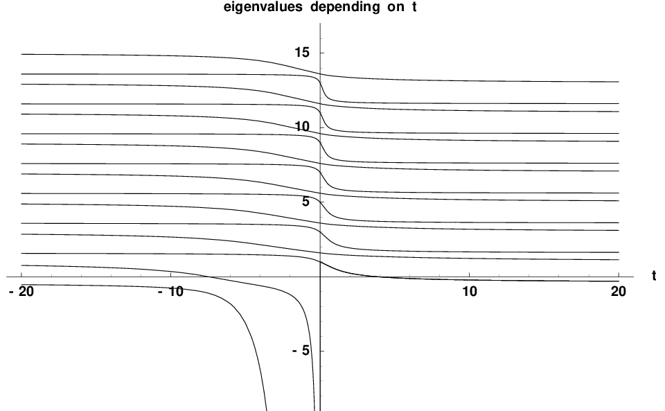
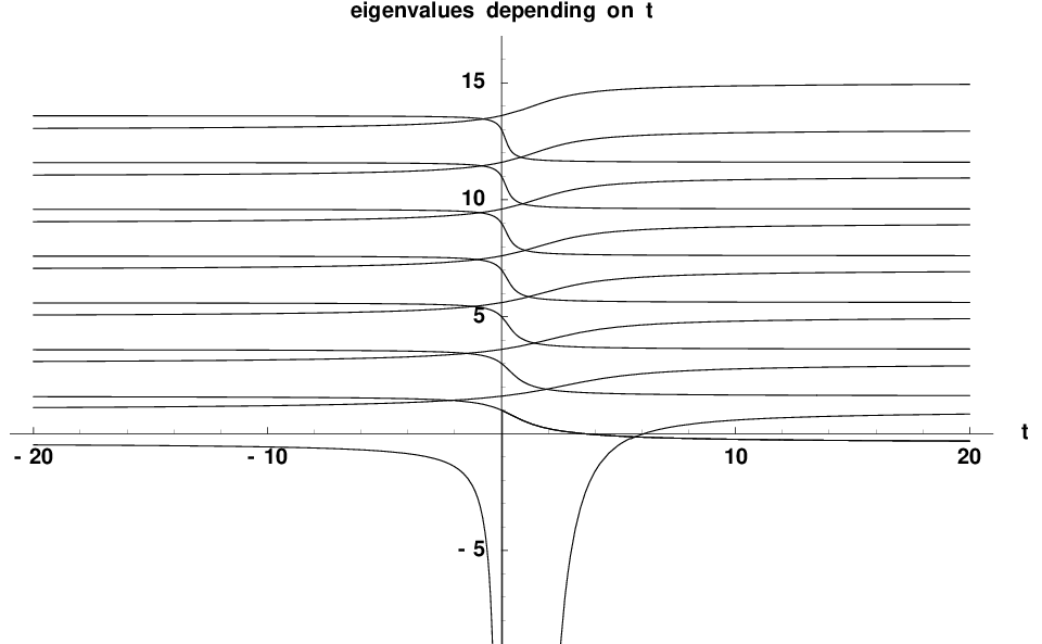
Instead we prefer to plot two graphs in order to give a reader some impression about how the eigenvalues may depend on the parameters, i.e. on the boundary conditions. In each graph we choose a line in the parameter space, {(ξ​t,η​t,ζ​t)∈ℝ3;t∈ℝ}\{(\xi t,\eta t,\zeta t)\in\mathbb{R}^{3};\ t\in\mathbb{R}\}, and we depict the dependence on tt of several first eigenvalues for the corresponding self-adjoint extension restricted to ℋc{\cal H}_{c} (see (22) for the substitution). In the both graphs we have set α=0.3\alpha=0.3 and B=1B=1.

Probably the most complete general information which is available about solutions of equation (23) might be a localisation of roots of this equation with respect to a suitable splitting of the real line into intervals. Let us choose the splitting into intervals with boundary points coinciding with the roots of equation (24). To get the localisation let us rewrite equation (23), equivalently provided z≠−ℤ+∪(1−α−ℤ+)z\neq-\mathbb{Z}_{+}\cup(1-\alpha-\mathbb{Z}_{+}), as follows

(Γ⁡(z−1+α)Γ⁡(z)+ξ)​(Γ⁡(z)Γ⁡(z+α)+η)=ζ2.\left(\frac{\Gamma(z-1+\alpha)}{\Gamma(z)}+\xi\right)\left(\frac{\Gamma(z)}{\Gamma(z+\alpha)}+\eta\right)=\zeta^{2}. (28)

Put

Fα​(z)=Γ⁡(z−1+α)Γ⁡(z)F_{\alpha}(z)=\frac{\Gamma(z-1+\alpha)}{\Gamma(z)}

so that equation (28) can be rewritten as

(Fα​(z)+ξ)​(F1−α​(z+α)+η)=ζ2.\left(F_{\alpha}(z)+\xi\right)\left(F_{1-\alpha}(z+\alpha)+\eta\right)=\zeta^{2}. (29)

It is easy to carry out some basic analysis of the function Fα​(z)F_{\alpha}(z). We have Fα′​(z)=Fα​(z)​(ψ⁡(z−1+α)−ψ⁡(z)){F_{\alpha}}^{\prime}(z)=F_{\alpha}(z)\,(\psi(z-1+\alpha)-\psi(z)). One observes that Fα​(z)>0F_{\alpha}(z)>0 for z∈]1−α,+∞[∪(⋃m∈ℤ+]−α−m,−m[)z\in{\,]1-\alpha,+\infty[\,}\,\cup\left(\bigcup_{m\in\mathbb{Z}_{+}}\,{\,]-\alpha-m,-m[\,}\right), and Fα​(z)<0F_{\alpha}(z)<0 for z∈⋃m∈ℤ+]−m,1−α−m[z\in\bigcup_{m\in\mathbb{Z}_{+}}\,{\,]-m,1-\alpha-m[\,}, and in any case Fα(z)′<0F_{\alpha}{}^{\prime}(z)<0. In the former case this follows from the fact that ψ⁡(z)\psi(z) is strictly increasing on each of the intervals ]0,+∞[{\,]0,+\infty[\,} and ]−m−1,−m[{\,]-m-1,-m[\,}, with m∈ℤ+m\in\mathbb{Z}_{+}. In the latter case this is a consequence of the identity

ψ⁡(z−1+α)−ψ⁡(z)=π​sin⁡(π​α)sin⁡(π​z)​sin⁡(π⁡(z+α))+∫0∞e−(1−z)​t​(1−e−(1−α)​t)1−e−t​𝑑t.\psi(z-1+\alpha)-\psi(z)=\frac{\pi\,\sin(\pi\alpha)}{\sin(\pi z)\,\sin(\pi(z+\alpha))}+\int_{0}^{\infty}\frac{e^{-\left(1-z\right)\,t}\left(1-e^{-\left(1-\alpha\right)\,t}\right)}{1-e^{-t}}\,\mathrm{d}t.

Moreover,

limz→+∞Fα(z)=0, limz→(1−α−m)±Fα(z)=±∞ and Fα(−m)=0 for m∈ℤ+.\lim_{z\rightarrow+\infty}F_{\alpha}(z)=0,\textrm{ }\lim_{z\rightarrow(1-\alpha-m)\pm}F_{\alpha}(z)=\pm\infty\textrm{ and }F_{\alpha}(-m)=0\textrm{ for }m\in\mathbb{Z}_{+}.

This also implies that F1−α​(z+α)>0F_{1-\alpha}(z+\alpha)>0 for z∈]0,+∞[∪(⋃m∈ℤ+]−1−m,−α−m[)z\in{\,]0,+\infty[\,}\,\cup\,\left(\bigcup_{m\in\mathbb{Z}_{+}}\,{\,]-1-m,-\alpha-m[\,}\right) and F1−α​(z)<0F_{1-\alpha}(z)<0 for z∈⋃m∈ℤ+]−α−m,−m[z\in\bigcup_{m\in\mathbb{Z}_{+}}\,{\,]-\alpha-m,-m[\,}, in any case F1−α(z+α)′<0F_{1-\alpha}{}^{\prime}(z+\alpha)<0, and

limz→+∞F1−α(z+α)=0, limz→−m±F1−α(z+α)=±∞,\displaystyle\lim_{z\rightarrow+\infty}F_{1-\alpha}(z+\alpha)=0,\textrm{ }\lim_{z\rightarrow-m\pm}F_{1-\alpha}(z+\alpha)=\pm\infty,
and ​F1−α​(−α−m)=0​ for ​m∈ℤ+.\displaystyle\textrm{and }F_{1-\alpha}(-\alpha-m)=0\textrm{ for }m\in\mathbb{Z}_{+}.

With the knowledge of these basic properties of the function Fα​(z)F_{\alpha}(z) it is a matter of an elementary analysis to determine the number of roots of equation (29) in each of the intervals ]1−α,+∞[{\,]1-\alpha,+\infty[\,}, ]−m,1−α−m[{\,]-m,1-\alpha-m[\,} and ]−α−m,−m[{\,]-\alpha-m,-m[\,}, with m∈ℤ+m\in\mathbb{Z}_{+}. The result is summarised in the following tables.

interval ]1−α,+∞[\,]1-\alpha,+\infty[\,
conditions number of roots
ξ≥0\xi\geq 0 η≥0\eta\geq 0 ζ2>ξ​η\zeta^{2}>\xi\eta 1
ξ≥0\xi\geq 0 η≥0\eta\geq 0 ζ2≤ξ​η\zeta^{2}\leq\xi\eta 0
ξ≥0\xi\geq 0 −Γ⁡(1−α)<η<0-\Gamma(1-\alpha)<\eta<0 no condition 1
ξ≥0\xi\geq 0 η≤−Γ⁡(1−α)\eta\leq-\Gamma(1-\alpha) no condition 0
ξ<0\xi<0 η≥0\eta\geq 0 no condition 1
ξ<0\xi<0 −Γ⁡(1−α)<η<0-\Gamma(1-\alpha)<\eta<0 ζ2≥ξ​η\zeta^{2}\geq\xi\eta 1
ξ<0\xi<0 −Γ⁡(1−α)<η<0-\Gamma(1-\alpha)<\eta<0 ζ2<ξ​η\zeta^{2}<\xi\eta 2
ξ<0\xi<0 η≤−Γ⁡(1−α)\eta\leq-\Gamma(1-\alpha) ζ2≥ξ​η\zeta^{2}\geq\xi\eta 0
ξ<0\xi<0 η≤−Γ⁡(1−α)\eta\leq-\Gamma(1-\alpha) ζ2<ξ​η\zeta^{2}<\xi\eta 1
interval ]0,1−α[\,]0,1-\alpha[\,
conditions number of roots
ξ≤0\xi\leq 0 η≥−Γ⁡(1−α)\eta\geq-\Gamma(1-\alpha) 0
ξ≤0\xi\leq 0 η<−Γ⁡(1−α)\eta<-\Gamma(1-\alpha) 1
ξ>0\xi>0 η≥−Γ⁡(1−α)\eta\geq-\Gamma(1-\alpha) 1
ξ>0\xi>0 η<−Γ⁡(1−α)\eta<-\Gamma(1-\alpha) 2
intervals ]−α−m,−m[\,]-\alpha-m,-m[\,, m∈ℤ+m\in\mathbb{Z}_{+}
conditions number of roots
ξ≥0\xi\geq 0 η≤0\eta\leq 0 0
ξ≥0\xi\geq 0 η>0\eta>0 1
ξ<0\xi<0 η≤0\eta\leq 0 1
ξ<0\xi<0 η>0\eta>0 2
intervals ]−1−m,−α−m[\,]-1-m,-\alpha-m[\,, m∈ℤ+m\in\mathbb{Z}_{+}
conditions number of roots
ξ≤0\xi\leq 0 η≥0\eta\geq 0 0
ξ≤0\xi\leq 0 η<0\eta<0 1
ξ>0\xi>0 η≥0\eta\geq 0 1
ξ>0\xi>0 η<0\eta<0 2

This is to be completed with the simple observation that 1−α1-\alpha is a root of (23) if and only if η=−Γ⁡(1−α)\eta=-\Gamma(1-\alpha), and −m-m, with m∈ℤ+m\in\mathbb{Z}_{+}, is a root if and only if ξ=0\xi=0, and finally −α−m-\alpha-m, with m∈ℤ+m\in\mathbb{Z}_{+}, is a root if and only if η=0\eta=0.

Let us note that this localisation is in agreement with a general result according to which if AA and BB are two self-adjoint extensions of the same symmetric operator with finite deficiency indices (d,d)(d,d) then any interval J⊂ℝJ\subset\mathbb{R} not intersecting the spectrum of AA contains at most dd eigenvalues of the operator BB (including multiplicities) and no other part of the spectrum of BB [12, §8.3]. Thus in our example if JJ is an open interval whose boundary points are either two subsequent eigenvalues of H∞H^{\infty} or the lowest eigenvalue of H∞H^{\infty} and −∞-\infty then any self-adjoint extension HΛH^{\Lambda} has at most two eigenvalues in JJ.

7 Concluding remarks

The above discussion does not exhaust all questions related to the system under consideration. One may ask, for instance, how the state of such a particle evolves under an adiabatic change of parameters. In particular, since the model exhibits eigenvalue crossings, one may expect that there are parameter loops exhibiting a nontrivial Berry phase. Another question concerns the physical meaning of our idealized model. More specifically, one is interested in which sense the model Hamiltonian can be approximated by those with smeared flux and a regular interaction. We leave these problems to a future publication.

Refer to caption
Figure 1: The Hamiltonian is determined by the boundary conditions corresponding to the parameters (ξ,η,ζ)=(0.95​t,0.25​t,0.25​t)(\xi,\eta,\zeta)=(0.95\,t,0.25\,t,0.25\,t), α=0.3\alpha=0.3, B=1B=1.
Refer to caption
Figure 2: The Hamiltonian is determined by the boundary conditions corresponding to the parameters (ξ,η,ζ)=(0.95​t,−0.25​t,0)(\xi,\eta,\zeta)=(0.95\,t,-0.25\,t,0), α=0.3\alpha=0.3, B=1B=1.

Acknowledgements. The research was partially supported by Grants GACR 201/01/01308 and GAAS 1018101.

References

  • [1] Y. Aharonov and D. Bohm: Significance of electromagnetic potentials in the quantum theory, Phys. Rev. 115 (1959) 485-491.
  • [2] S. N. M. Ruijsenaars: The Aharonov-Bohm effect and scattering theory, Annals Phys. 146 (1983) 1-34.
  • [3] H.-P. Thienel: Quantum mechanics of an electron in a homogeneous magnetic field and a singular magnetic flux tube, Annals Phys. 280 (2000) 140-162.
  • [4] R. M. Cavalcanti: Comment on “Quantum mechanics of an electron in a homogeneous magnetic field and a singular magnetic flux tube”, quant-ph/0003148.
  • [5] M. Hirokawa, O. Ogurisu: Ground state of a spin 1/2 charged particle in a two-dimensional magnetic field, J. Math. Phys. 42 (2001) 3334-3343.
  • [6] S. Albeverio, F. Gesztesy, R. Høegh-Krohn and H. Holden: Point interactions in two dimensions: Basic properties, approximations and applications to solid state physics, J. reine angew. Math. 380 (1987) 87-107.
  • [7] L. Da̧browski and P. Šťovíček: Aharonov-Bohm effect with δ\delta-type interaction, J. Math. Phys. 39 (1998) 47-62.
  • [8] R. Adami and A. Teta: On the Aharonov-Bohm Hamiltonian, Lett. Math. Phys. 43 (1998) 43.
  • [9] M. Abramowitz, I.A. Stegun: Handbook of Mathematical Functions with Formulas, Graphs and Mathematical Tables, Dover Publications, New York, 1965.
  • [10] A.P. Prudnikov, J.A. Bryčkov and O.I. Maričev: Intěgraly i rjady, Nauka, Moskva, 1986.
  • [11] M. Reed and B. Simon: Methods of Modern Mathematical Physics IV, Academic, New York, 1975.
  • [12] J. Weidmann: Linear Operators in Hilbert Spaces, Springer-Verlag, New York, 1980.