Exact and Approximate Performance of Concatenated Quantum Codes

Quantum Error Correction Nielsen and Chuang 2000 and Fault-Tolerant Computation Preskill 1997 have demonstrated that, in principle, quantum computing is possible despite noise in the computing device. Analyses in these areas, as in many physics disciplines, rely on asymptotic limits and expansions in small parameters. However, realistic devices will be of large but finite scale and real parameter values may not be sufficiently small; thus methods valid outside these limits are desirable. Here we demonstrate the use of model reduction Dullerud and Paganini 2000; Rahn, a control theory technique, for studying large but finite quantum systems.

We will first derive the effective channel describing an encoded qubit’s evolution under arbitrary error dynamics, and propagate these results to concatenation schemes Nielsen and Chuang 2000 when the dynamics do not couple code blocks. The calculations for both finite and asymptotic concatenation are simple, but the resulting expressions for the effective channel dynamics in the finite case are cumbersome and ill-conditioned. We will then use model reduction to find low-order approximations for these dynamics. Among other results, we derive a model for a $9^{4}$-qubit system requiring only 23 degrees of freedom for accuracy $\sim 10^{-3}$.

We consider the following formulation of quantum error correction: a single-qubit state $\rho_{0}$ is perfectly encoded in a multi-qubit register with state $\rho$, which evolves via some error dynamics described by a linear map $\rho(0)\mapsto\rho(t)=\mathcal{E}[\rho(0)]$. (For master equation evolution $\dot{\rho}=\mathcal{L}[\rho]$, $\mathcal{E}=e^{\mathcal{L}t}$.) At time $t$, a syndrome measurement is made and the appropriate recovery operator is performed; we assume the measurement and recovery are noiseless. This process returns the system to the codespace ¹¹ 1 We may choose such a recovery procedure even if the code is imperfect., and thus its state can be described by a single-qubit state $\rho_{f}$. Denote the probability-weighted average of $\rho_{f}$ over syndrome measurement outcomes by $\overline{\rho_{f}}$. For a given code and error model, we wish to know $\overline{\rho_{f}}(t)$: we may then compare $\rho_{0}$ and $\overline{\rho_{f}}(t)$ via a desired fidelity measure.

The logical qubit $\rho_{0}$ may be parameterized by the expectation values $\langle I\rangle_{0}$, $\langle X\rangle_{0}$, $\langle Y\rangle_{0}$ and $\langle Z\rangle_{0}$, with $\{I,X,Y,Z\}$ the usual Pauli matrices. (Of course $\langle I\rangle=1$, but it will be convenient to include this term.) The logical qubit $\rho_{0}$ is encoded by preparing the register in the state $\rho(0)=\langle I\rangle_{0}E_{I}+\langle X\rangle_{0}E_{X}+\langle Y\rangle_{0}E_{Y}+\langle Z\rangle_{0}E_{Z}$ where $E_{\sigma}$ acts as $\frac{1}{2}\sigma$ on the two-dimensional codespace and vanishes elsewhere. These operators are easily constructed from the codewords: for example, given the encoding $|0\rangle\mapsto|\overline{0}\rangle$, $|1\rangle\mapsto|\overline{1}\rangle$, we have $E_{X}=\frac{1}{2}(|\overline{0}\rangle\langle\overline{1}|+|\overline{1}\rangle\langle\overline{0}|)$. (For a stabilizer code Nielsen and Chuang 2000 with stabilizer $S=\{S_{i}\}$ and logical operators $\bar{\sigma}$, the codespace projector is $P_{C}=\frac{1}{|S|}\sum_{i}S_{i}$ and $E_{\sigma}=\frac{1}{2}P_{C}\bar{\sigma}$.) E.g., for the bitflip code Nielsen and Chuang 2000 given by $|0\rangle\mapsto|000\rangle$, $|1\rangle\mapsto|111\rangle$,

For the trivial code ($\rho_{0}$ “encoded” as itself in a single-qubit register) we have simply $E_{\sigma}=\frac{1}{2}\sigma$.

After the action of $\mathcal{E}$, recovery yields the expected logical state $\overline{\rho_{f}}$. As with $\rho_{0}$, we parameterize $\overline{\rho_{f}}$ by the expectation values $\langle I\rangle_{{\bar{f}}}$, $\langle X\rangle_{{\bar{f}}}$, $\langle Y\rangle_{{\bar{f}}}$ and $\langle Z\rangle_{{\bar{f}}}$. The $\langle\sigma\rangle_{{\bar{f}}}$ may be written as expectation values of operators on the register prior to recovery: letting $\{P_{j}\}$ be the syndrome measurement projectors and $\{R_{j}\}$ be the recovery operators, $\langle\sigma\rangle_{{\bar{f}}}=\mathrm{tr}(D_{\sigma}\rho)$ where $D_{\sigma}=2\sum_{j}P_{j}^{\dagger}R_{j}^{\dagger}E_{\sigma}R_{j}P_{j}$. (For a stabilizer code, $R_{j}$ is some Pauli operator of lowest weight leading to syndrome measurement $P_{j}$, and $D_{\sigma}=\frac{1}{|S|}\sum_{i}f_{i\sigma}S_{i}\bar{\sigma}$, with $f_{i\sigma}=\sum_{j}\eta(S_{i},R_{j})\eta(R_{j},\bar{\sigma})$ where $\eta(p,q)=\pm 1$ for $pq=\pm qp$.) For the bitflip code,

For the trivial code we have simply $D_{\sigma}=\sigma$.

To describe the evolution of the encoded logical bit, we compute the effective channel $\mathcal{G}$ taking $\rho_{0}$ to $\overline{\rho_{f}}$. $\mathcal{G}$ may be written as the linear mapping of $\vec{\rho}_{0}=(\langle I\rangle_{0},\langle X\rangle_{0},\langle Y\rangle_{0},\langle Z\rangle_{0})$ to $\vec{\rho}_{\bar{f}}=(\langle I\rangle_{\bar{f}},\langle X\rangle_{\bar{f}},\langle Y\rangle_{\bar{f}},\langle Z\rangle_{\bar{f}})$:

If $\mathcal{E}$ is completely positive Nielsen and Chuang 2000, it follows that $\mathcal{G}$ is as well.

To obtain a matrix representation of $\mathcal{G}$, let

Then $\vec{\rho}_{\bar{f}}=\mathcal{G}\vec{\rho}_{0}$, and the fidelity of a pure logical qubit under this process is $\frac{1}{2}\vec{\rho}_{0}^{\>{\mathrm{T}}}\mathcal{G}\vec{\rho}_{0}$. Note that the dynamics $\mathcal{E}$ need not be those against which the code protects.

Now consider concatenated codes Nielsen and Chuang 2000. In the concatenation of two codes, a qubit is encoded using the outer code $C^{\mathrm{out}}$ and then each of the resulting qubits is encoded using the inner code $C^{\mathrm{in}}$. Though not necessarily optimal, a simple error-correction scheme coherently corrects each of the inner code blocks, and then corrects the entire register based on the outer code. We denote the concatenated code (with this correction scheme) by $C^{\mathrm{out}}(C^{\mathrm{in}})$. Given the effective channel $\mathcal{G}$ describing $C^{\mathrm{in}}$ under some dynamics, and a desired $C^{\mathrm{out}}$, we now construct $\widetilde{\mathcal{G}}$ describing the evolution under $C^{\mathrm{out}}(C^{\mathrm{in}})$.

Let $C^{\mathrm{out}}$ be an $N$-bit code and $C^{\mathrm{in}}$ be an $M$-bit code. We assume that each $M$-bit block evolves according to the original dynamics $\mathcal{E}$ and no cross-block correlations are introduced, thus the evolution operator is $\widetilde{\mathcal{E}}=\mathcal{E}\otimes\mathcal{E}\otimes\ldots\otimes\mathcal{E}$. Each $M$-bit block represents a single logical qubit encoded in $C^{\mathrm{in}}$; as the block has dynamics $\mathcal{E}$, this logical qubit’s evolution is described by $\mathcal{G}$. Therefore the effective evolution operator for the logical bits in the codeword of $C^{\mathrm{out}}$ is $\widetilde{\mathcal{E}}_{\mathrm{eff}}=\mathcal{G}\otimes\mathcal{G}\otimes\ldots\otimes\mathcal{G}.$

Operators on $N$ qubits may be written as sums of tensor products of $N$ Pauli matrices; we may therefore write

(For stabilizer codes, the $\alpha$ and $\beta$ coefficients are easily found.) Substituting $\widetilde{\mathcal{E}}_{\mathrm{eff}}$, $E^{\mathrm{out}}_{\sigma^{\prime}}$ and $D^{\mathrm{out}}_{\sigma}$ into (4) and noting that $\mathrm{tr}(\nu_{j}\mathcal{G}[\frac{1}{2}\mu_{j}])=\mathcal{G}_{\nu_{j}\mu_{j}}$ yields

Thus the matrix elements of $\widetilde{\mathcal{G}}$ can be expressed as polynomials of the matrix elements of $\mathcal{G}$, with the polynomial coefficients $\beta_{\{\nu_{i}\}}^{\sigma}\alpha_{\{\mu_{i}\}}^{\sigma^{\prime}}$ depending only on the $E_{\sigma}$ and $D_{\sigma}$ of the outer code. For a given outer code $C$, denote the concatenation map $\mathcal{G}\mapsto\widetilde{\mathcal{G}}$ by $\Omega^{C}$. It can be shown that $\Omega^{C}$ preserves complete positivity.

More generally, the inner process $\mathcal{G}$ can represent any linear evolution of a logical qubit, and thus we may speak of concatenating a qubit process with a code. E.g., if $\mathcal{G}$ describes some qubit dynamics, then $\Omega^{C}(\mathcal{G})$ describes the effective dynamics of encoding by $C$ with the uncorrelated dynamics $\mathcal{G}$ acting on each register bit. This method only requires that the outer code’s logical qubits be decoupled. (Above we assumed $\widetilde{\mathcal{E}}_{\mathrm{eff}}=\mathcal{G}\otimes\ldots\otimes\mathcal{G}$; for $\widetilde{\mathcal{E}}_{\mathrm{eff}}=\mathcal{G}^{(1)}\otimes\ldots\otimes\mathcal{G}^{(N)}$, replace $\mathcal{G}_{\nu_{j}\mu_{j}}$ with $\mathcal{G}^{(j)}_{\nu_{j}\mu_{j}}$ in (7).)

We may characterize both the finite and asymptotic behavior of any concatenation scheme involving the codes $\{C_{k}\}$ by computing the maps $\Omega^{C_{k}}$. Then the finite concatenation scheme $C_{1}(C_{2}(\ldots C_{n}\ldots))$ is characterized by $\Omega^{C_{1}(C_{2}(\ldots C_{n}\ldots))}=\Omega^{C_{1}}(\Omega^{C_{2}}(\ldots\Omega^{C_{n}}\ldots))$. We expect the typical $\Omega^{C}$ to be sufficiently well-behaved that standard dynamical systems methods Devaney 1989 will yield the $\ell\rightarrow\infty$ limit of $(\Omega^{C})^{\ell}$; one need not compose the $(\Omega^{C})^{\ell}$ explicitly.

We now consider certain concatenation schemes when the symmetric depolarizing channel Nielsen and Chuang 2000 acts on each register qubit. This channel is described by $\mathcal{G}^{\mathrm{dep}}(t)$ diagonal with entries $(1,e^{-\gamma t},e^{-\gamma t},e^{-\gamma t})$. From trace preservation $\mathcal{G}_{II}$ is always 1, so let $[x,y,z]$ denote $\mathcal{G}$ diagonal with entries $(1,x,y,z)$; then $\mathcal{G}^{\mathrm{dep}}(t)=[e^{-\gamma t},e^{-\gamma t},e^{-\gamma t}]$.

Suppose more generally we are given a qubit process described by $\mathcal{G}=[x,y,z]$, and wish to concatenate this process with the bitflip (bf) code. Using (7) and the coding operators (1) and (2), we find that $\Omega^{\mathrm{bf}}(\mathcal{G})$ describing the concatenated evolution is also diagonal:

((8) could also be found by using the Heisenberg picture to evaluate (4).) Writing $|\pm\rangle=\frac{1}{\sqrt{2}}(|0\rangle\pm|1\rangle)$, the map $\Omega^{\mathrm{pf}}$ for the phaseflip code $|\pm\rangle\mapsto|\!\pm\!\pm\pm\rangle$ Nielsen and Chuang 2000 is similar. (Any stabilizer code $C_{S}$ preserves diagonality: $\Omega^{C_{S}}([x,y,z])$ is

with $w_{\sigma}(p)$ the $\sigma$-weight of a Pauli operator $p$ (e.g. $w_{X}(XYX)=2$) and $f_{i\sigma}$ as previously defined.)

The concatenation phaseflip(bitflip) yields the encoding $|\pm\rangle\mapsto\frac{1}{\sqrt{8}}(|000\rangle\pm|111\rangle)^{\otimes 3}$, which is the Shor nine-bit code Nielsen and Chuang 2000. Thus $\Omega^{\mathrm{Shor}}=\Omega^{\mathrm{pf}}(\Omega^{\mathrm{bf}})$, and $\Omega^{\mathrm{Shor}}([x,y,z])=$

Now consider the Shor code concatenated with itself $\ell$ times, and let $[\widetilde{x}_{\ell}(t),\widetilde{y}_{\ell}(t),\widetilde{z}_{\ell}(t)]=(\Omega^{\mathrm{Shor}})^{\ell}(\mathcal{G}^{\mathrm{dep}}(t))$. The functions $\widetilde{\sigma}_{\ell}(t)$ approach step functions in the limit $\ell\rightarrow\infty$ (e.g., see Fig. 1); denote these step functions’ times of discontinuity by $t_{\sigma}^{\star}$. Thus in the infinite concatenation limit, the code will perfectly protect the $\langle\sigma\rangle$ component of the logical qubit if correction is performed prior to $t_{\sigma}^{\star}$. We call $t_{\sigma}^{\star}$ the $\sigma$-storage threshold.

We calculate the $t_{\sigma}^{\star}$ by finding the $\ell\rightarrow\infty$ limit of $\widetilde{\sigma}_{\ell}(t)$. Writing (Exact and Approximate Performance of Concatenated Quantum Codes) as $[Q_{1}(x)$, $Q_{2}(x,y,z),Q_{3}(z)]$, the map $z\mapsto Q_{3}(z)$ has stable fixed points at 0 and 1 and one unstable fixed point $z^{\star}$ on $(0,1)$; numerically solving $Q_{3}(z)=z$ yields $z^{\star}\approx 0.730$. The plots of $\widetilde{z}_{\ell}(t)$ all intersect at $\widetilde{z}(t_{Z}^{\star})=z^{\star}$, and the step function limit follows from the stability of 0 and 1. Inverting $e^{-\gamma t}=z^{\star}$ yields $t_{Z}^{\star}$. $Q_{1}$ has similar features with $x^{\star}\approx 0.900$, and a similar analysis yields $t_{X}^{\star}$. For this code, one can show $t_{Y}^{\star}=\min(t_{X}^{\star},t_{Z}^{\star})$.

We may also phrase the thresholds in the language of finitely probable errors. The expected evolution of a qubit subjected to a random Pauli error with probability $p$ is $\rho\mapsto(1-p)\rho+\frac{p}{3}X\rho X+\frac{p}{3}Y\rho Y+\frac{p}{3}Z\rho Z$. This channel is described by $\mathcal{G}^{\mathrm{Pauli}}(p)=[1-\frac{4}{3}p,1-\frac{4}{3}p,1-\frac{4}{3}p]$. As $\mathcal{G}^{\mathrm{Pauli}}(\frac{3}{4}(1-e^{-\gamma t}))=\mathcal{G}^{\mathrm{dep}}(t)$, in the infinite concatenation limit with $\mathcal{G}^{\mathrm{Pauli}}(p)$ acting on each register qubit, the logical qubit’s $\langle\sigma\rangle$ component will be perfectly protected if $p<p^{\star}_{\sigma}=\frac{3}{4}(1-e^{-\gamma t^{\star}_{\sigma}})$. Define the threshold probability $p_{\mathrm{th}}=\min\{p^{\star}_{\sigma}\}$; for $p<p_{\mathrm{th}}$, all encoded qubits are perfectly protected in the infinite concatenation limit. Values for $t^{\star}_{\sigma}$ and $p_{\mathrm{th}}$ appear in Table 1.

For comparison, we derived thresholds for three other codes. Another version of the Shor code is given by $|0\rangle\mapsto\frac{1}{\sqrt{8}}(|000\rangle+|111\rangle)^{\otimes 3}$, $|1\rangle\mapsto\frac{1}{\sqrt{8}}(|000\rangle-|111\rangle)^{\otimes 3}$; call this code Shor^′. Let $[\widetilde{x}^{\prime}_{\ell}(t),\widetilde{y}^{\prime}_{\ell}(t),\widetilde{z}^{\prime}_{\ell}(t)]=(\Omega^{\mathrm{Shor}^{\prime}})^{\ell}(\mathcal{G}^{\mathrm{dep}}(t))$. The $\widetilde{y}^{\prime}_{\ell}(t)$ approach a step function as $\ell\rightarrow\infty$, but $\widetilde{x}^{\prime}_{\ell}(t)$ and $\widetilde{z}^{\prime}_{\ell}(t)$ approach a limit cycle of period 2, interchanging step functions with different discontinuities at every iteration of $\Omega^{\mathrm{Shor}^{\prime}}$. Considering instead the limit of iterating $(\Omega^{\mathrm{Shor}^{\prime}})^{2}$ permits an analysis as for $\Omega^{\mathrm{Shor}}$. The Steane seven-bit code Nielsen and Chuang 2000 may be treated similarly to the Shor code, and the symmetries of the Five-Bit code Nielsen and Chuang 2000 lead to a simple analysis. Results are summarized in Table 1.

We now return to the Shor code under the depolarizing channel, and consider the finite concatenations described by the functions $\widetilde{\sigma}_{\ell}(t)$. The $\widetilde{\sigma}_{\ell}(t)$ have the form $\sum_{i}b_{i}e^{-a_{i}\gamma t}$ with the $a_{i}$ positive integers and the $b_{i}$ rationals. For $\gamma=0$ no errors occur, thus $\sum_{i}b_{i}=1$.

Explicit calculation of the $\widetilde{\sigma}_{\ell}$ has several disadvantages. First, the number of terms in these series grows approximately as $9^{\ell}$ (see Table 2(a)). Though not nearly as severe as for the number of elements in the full-system density matrix ($2^{2\cdot 9^{\ell}}$), this growth is still too rapid to be practical. Only a small portion of the terms in these series have $|b_{i}|<1$, thus one cannot meaningfully truncate the series without introducing significant error.

More seriously, the magnitude of the $b_{i}$ grows rapidly: e.g., $|b_{i}|>10^{60}$ for 65 of the 352 terms in $\widetilde{z}_{3}$, and double-floating point precision no longer yields $\sum_{i}b_{i}=1$. To efficiently generate plots of the $\widetilde{\sigma}_{\ell}(t)$ we repeatedly apply $\Omega^{\mathrm{Shor}}$ to numerical values of $[e^{-\gamma t},e^{-\gamma t},e^{-\gamma t}]$ for all desired times $t$. However, this leaves us without a dynamic model for the evolution of $\overline{\rho_{f}}(t)$.

Given $\mathcal{G}(t)=[\widetilde{x}(t),\widetilde{y}(t),\widetilde{z}(t)]$, for each $\widetilde{\sigma}(t)$ we will seek a square matrix $A_{\sigma}$, column vector $B_{\sigma}$ and row vector $C_{\sigma}$ such that $\widetilde{\sigma}(t)\approx C_{\sigma}e^{A_{\sigma}t}B_{\sigma}$. For $n\times n$ $A_{\sigma}$, we say $(A_{\sigma},B_{\sigma},C_{\sigma})$ is an order $n$ realization of $\widetilde{\sigma}(t)$. (These methods may be generalized to non-diagonal $\mathcal{G}(t)$ by seeking matrices $A$, $B$ and $C$ of sizes $n\times n$, $n\times 4$ and $4\times n$ respectively such that $\mathcal{G}(t)\approx Ce^{At}B$.) For $\widetilde{\sigma}(t)=\sum_{i}b_{i}e^{-a_{i}\gamma t}$, we can exactly realize $\widetilde{\sigma}(t)$ by choosing $A_{\sigma}$ diagonal with entries $-a_{i}\gamma$, $B_{\sigma}$ with entries $b_{i}$, and $C_{\sigma}=(1,1,\dots,1)$. If the $a_{i}$ are distinct and the $b_{i}$ non-zero, this realization is minimal: there is no lower-order exact realization of $\widetilde{\sigma}(t)$.

To find approximate lower-order realizations we use the model reduction technique of balanced truncation Dullerud and Paganini 2000; Rahn. Consider a system with time-varying input $u(t)\in\mathbb{R}$, state $x(t)\in\mathbb{R}^{n}$, dynamics $\dot{x}=Ax+Bu$, and output $y(t)=Cx\in\mathbb{R}$; if $u=\delta(t)$, $y=Ce^{At}B$ for $t>0$. Note that $(A,B,C)\rightarrow(TAT^{-1},TB,CT^{-1})$ leaves the map $\Psi:u(t)\mapsto y(t)$ unchanged. An arbitrary truncation of state-space dimensions, e.g. $\left(\left[\genfrac{}{}{0.0pt}{}{a_{11}}{a_{21}}\genfrac{}{}{0.0pt}{}{a_{12}}{a_{22}}\right],\left[\genfrac{}{}{0.0pt}{}{b_1}{b_2}\right],[c_{1}\>c_{2}]\right)\rightarrow([a_{11}],[b_{1}],[c_{1}])$, may yield a radically different map $\Psi$. However, we may numerically construct a balancing transformation $T$ such that in the balanced system, a non-negative real Hankel Singular Value (HSV) $h_{i}$ is associated with each dimension of the state-space $\mathbb{R}^{n}$. Removing all dimensions with $h_{i}=0$ yields a minimal realization; further truncating dimensions with small HSVs introduces a small error in $\Psi$ which, in an appropriate norm, is bounded by the sum of the truncated HSVs ²² 2 Balanced truncation for $u=\delta(t)$ will be discussed elsewhere..

Writing the series for $\widetilde{\sigma}(t)$ as minimal realizations, we can balance and calculate their HSVs. In Fig. 2 we see the HSVs for $\widetilde{z}(t)$ after each level of bitflip and phaseflip concatenation up to pf(bf(pf(bf))) = Shor². Note that the number of non-zero HSVs grows rapidly at each level of concatenation, but the number of HSVs above any $h_{\mathrm{min}}$ grows slowly. ($\widetilde{x}(t)$ and $\widetilde{y}(t)$ give similar results.)

Consider $\widetilde{z}_{2}(t)$, with minimal realization of order 37: the first five HSVs are $(2.5\times 10^{-1})/\gamma$, $(3.7\times 10^{-2})/\gamma$, $(5.3\times 10^{-3})/\gamma$, $(6.0\times 10^{-4})/\gamma$, and $(5.4\times 10^{-5})/\gamma$. Truncating all but the four most significant dimensions yields an approximation almost indistinguishable from the exact $\widetilde{z}_{2}(t)$; truncating further to realizations of order 3 and 2 only mildly degrades the approximation (see Fig. 3).

Given realizations for the $\widetilde{\sigma}(t)$, we may construct realizations for polynomials of the $\widetilde{\sigma}(t)$ as follows. Given $f(t)=C_{f}e^{A_{f}t}B_{f}$ and $g(t)=C_{g}e^{A_{g}t}B_{g}$, the function $f(t)g(t)$ is realized by $(A_{f}\otimes\openone+\openone\otimes A_{g},B_{f}\otimes B_{g},C_{f}\otimes C_{g})$. The function $f(t)+g(t)$ is realized by $\left(\left[\genfrac{}{}{0.0pt}{}{A_f}{}\genfrac{}{}{0.0pt}{}{}{A_g}\right],\left[\genfrac{}{}{0.0pt}{}{B_f}{B_g}\right],[C_{f}\>\>C_{g}]\right)$. For a scalar $\alpha$, the function $\alpha f(t)$ is realized by $(A_{f},B_{f},\alpha C_{f})$. Composing these operations allows any polynomial of the $\widetilde{\sigma}(t)$ to be realized, and thus we may directly apply the $\Omega^{C}$ to realizations.

For $\ell>2$ it is impractical to construct the exact $\widetilde{\sigma}_{\ell}(t)$ and then apply balanced truncation. Instead, we build approximate realizations for the $\widetilde{\sigma}_{\ell}(t)$ using an iterative approach. Begin with minimal realizations for the $\widetilde{\sigma}_{0}(t)$ describing $\mathcal{G}^{\mathrm{dep}}(t)$. Alternately apply $\Omega^{\mathrm{bf}}$ and $\Omega^{\mathrm{pf}}$ to these realizations; after each concatenation, balance and truncate dimensions with HSVs less than some $h_{\mathrm{min}}$. Choosing $h_{\mathrm{min}}=(4\times 10^{-5})/\gamma$ yields realizations with orders shown in Table 2(b). Comparing to Table 2(a), we see the resulting order reduction is dramatic.

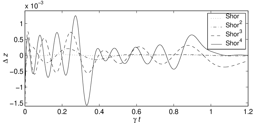
Fig. 4 shows the differences between the exact $\widetilde{z}_{\ell}(t)$ and the results of the iterative reduction method. Results for approximating $\widetilde{x}_{\ell}(t)$ and $\widetilde{y}_{\ell}(t)$ are similar. Up to eight 3-qubit concatenations, the worst errors $|\Delta\widetilde{\sigma}_{\ell}(t)|$ are only $\approx 3\times 10^{-3}$. Note that the errors appear to have characteristic frequencies; the error is analogous to the ringing in frequency-limited approximations of step functions. To good accuracy the mutual intersection points of the $\widetilde{x}_{\ell}(t)$ and of the $\widetilde{z}_{\ell}(t)$ are preserved; this is expected as the concatenation polynomials are unchanged.

These results suggest balanced truncation is a powerful approximation tool in quantum settings. Future work will further investigate the iterative reduction method, and attempt to find bounds on the approximation errors.