Quantum Nonlocality for a Mixed Entangled Coherent State

Einstein, Podolsky, and Rosen proposed a thought experiment to test the local realism properties of quantum mechanics [1]. An inequality imposed by a local hidden variable theory was suggested by Bell [2], which enables a quantitative test concerning the controversy of local realism versus quantum mechanics in a real laboratory. Various versions of Bell’s inequality [3, 4] followed the original one, and experiments have been performed testing local realism [5]. In spite of successful experimental results, it has been pointed out that there remain two possible loopholes. One is called the lightcone loophole that might allow local realistic interpretation. Some experiments have been performed with strict relativistic separation between measurements to close this loophole [6]. The other is the detection loophole due to detection inefficiency. According to this loophole, there is a possibility that the detected subensemble violates Bell’s inequality even though the whole ensemble satisfies it. Some authors generalised Bell’s inequality to the case of inefficient detection [4, 7, 8] and other proposals have been made [9] to close the detection loophole. An experiment on nonlocality has been performed with an efficient detection [10].

The nonlocality test can be performed on an entangled system composed of two coherent systems [11]. This entangled system can be used as a quantum entangled channel for quantum information transfer. The entangled coherent state can be generated using a coherent light propagating through a nonlinear medium [12] and a 50-50 beam splitter as shown in Fig. 1. There have also been proposals to entangle fields in two spatially separated cavities [13]. The entangled coherent state and its usage for quantum information processing [14, 15, 16, 17], teleportation [14, 16, 17] and entanglement concentration [17] have all been studied recently.

In this paper, we study nonlocality of an entangled coherent state using photon parity measurement. We first investigate the nonlocality of a pure entangled coherent state, and move on to the dynamic behavior of nonlocality for a decohered entangled coherent state in a vacuum environment. The dynamic behaviour is also investigated in the framework of $2\times 2$ Hilbert space and the results are compared. It is found that nonlocality of a decohered entangled coherent sate persists longer when it is considered in $2\times 2$ space.

We are interested in nonlocality of an entangled coherent state

where $\alpha=\alpha_{r}+i\alpha_{i}$ is a complex amplitude, $\varphi$ is a real local phase factor, and $N$ is a normalisation factor. By applying local unitary transformations any state in the form of

with arbitrary amplitudes $\beta$ and $\gamma$ can be transformed to a form like that of Eq. (1) up to a global phase factor. Applying displacement operators $D_{1}(x)D_{2}(x)$, where $x=x_{r}+ix_{i}$ is complex, the entangled coherent state (2) becomes

with $x=-\frac{1}{2}(\beta+\gamma)$, $\alpha=\beta+x=-(\gamma+x)$, and $\phi=x_{i}\beta_{r}-x_{r}\beta_{i}+x_{i}\alpha_{r}-x_{r}\alpha_{i}$. Here the displacement operator is defined as $D(x)=\exp(xa^{\dagger}+x^{*}a)$, where $a$ and $a^{\dagger}$ are annihilation and creation operators [18]. In this paper, we consider the nonlocality of entangled coherent states

where $N_{\pm}$ are normalisation factors and $\alpha$ is assumed to be real for simplicity.

The type of quantum observable to be measured is a crucial factor in the nonlocality test. Banaszek and Wódkiewicz developed a Wigner function representation of the Bell-Clauser, Horne, Shimony and Holt (CHSH) [3] inequality using a two-mode parity operator $\Pi(\alpha,\beta)$ as a quantum observable [19, 20]. The two-mode parity operator $\Pi(\alpha,\beta)$ is defined as

where

with

The Bell-CHSH inequality is then

where we call $|{\cal B}|$ the Bell measure. The displacement operation can be effectively performed using a beam splitter with the transmission coefficient close to one and a strong coherent state being injected into the other input port [20]. The two-mode Wigner function at a given phase point described by $\alpha$ and $\beta$ is

where $\rho$ is the density operator of the field. From Eqs.(8) and (9), we obtain the Wigner representation of Bell’s inequality

The Wigner function of an entangled coherent state is obtained from the Fourier transform of it’s characteristic function

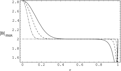
Banaszek and Wódkiewicz used their Wigner function based Bell measure with $\alpha=\beta=0$. We consider all four variables $\alpha,\beta,\alpha^{\prime}$ and $\beta^{\prime}$ in our investigation of the Wigner function based Bell measure as shown in Eq. (10) to test nonlocality more generally. The maximum Bell-CHSH violation using Banaszek and Wódkiewicz’s version is approximately 2.19 for two-mode squeezed states [19, 22] and 2.5 for entangled coherent states as shown in Fig. 2. However, for the generalised Bell measure in Eq. (10), both two-mode squeezed states [23] and entangled coherent states have a maximal Bell-CHSH violation of $2\sqrt{2}$ (as shown in Fig. 2).

The entangled coherent states $|C_{-}\rangle$ and $|C_{+}\rangle$ violate the Bell inequality regardless of the size of the amplitude, $\alpha>0$. As the amplitude $\alpha$ increases the Bell measure tends towards a maximum of $2\sqrt{2}$.

It is interesting to note that the Bell measure for the $|C_{-}\rangle$ state takes a higher value than for the $|C_{+}\rangle$ state. If the number state representation of the coherent state is [18]

which means that, in the limit of small coherent amplitude $\alpha$,

Substituting this into the entangled coherent states $|C_{+}\rangle$ and $|C_{-}\rangle$ we find

When $\alpha$ is small $|C_{+}\rangle\rightarrow|0\rangle|0\rangle$. As the weights of $|0\rangle|0\rangle$ and $|1\rangle|1\rangle$ are radically different $|C_{+}\rangle$ is only minimally entangled. However the two component states $|0\rangle|1\rangle$ and $|1\rangle|0\rangle$ are equally weighted for $|C_{-}\rangle$ which gives optimal entanglement. A pure entangled state always violates nonlocality [24]. Any entangled coherent state in a form as given in Eq. (4) is found to be nonlocal. We conjecture that any entangled coherent state as given in Eq. (2) also has nonlocality except when $\beta=\gamma$, i.e., when the state is a product state.

The results shown in Fig. 2 were obtained from a numerical consideration of the Bell measure (10). In analogy with the work carried out in [22] we imposed the condition $\cal{B}(|\alpha|,|\beta|,|\alpha^{\prime}|,|\beta^{\prime}|)=\cal{B}(|\beta|,|\alpha|,|\beta^{\prime}|,|\alpha^{\prime}|)$. The method of steepest descent [25] was used to find the maximum of the Bell measure under our assumptions.

A quantum system loses its quantum characteristics if it is open to the world. We modelled an entangled coherent state interacting with a dissipative environment (two independent vacuum reservoirs). To study the dynamics of nonlocality of continuous variable entangled coherent states it is necessary to find an expression of the time-dependent Bell-CHSH measure. This in turn means finding an expression for the time-dependent decohered Wigner function.

The quantum channel decoheres when it interacts with it’s environment and becomes a mixed state of its density operator $\rho(\tau)$, where $\tau$ is the decoherence time. To know the time dependence of $\rho(\tau)$, we have to solve the master equation

where $a_{i}$ and $a_{i}^{\dagger}$ are the annihilation and creation operators for the field mode $i$ and $\gamma$ is the decay constant. We have assumed that each field mode is coupled to its environment at the same coupling rate $\gamma$. The formal solution of the master equation (15) can be written as

which leads to the solution for the initial single-mode dyadic $|\alpha\rangle\langle\beta|$

where $t=e^{-\frac{1}{2}\gamma\tau}$. In this paper, we introduce a dimensionless normalised interaction time $r$ which is related to $t$ by the expression $r=\sqrt{1-t^{2}}$. When $\tau=0,t=1$ and $r=0$. As $\tau\rightarrow\infty,t\rightarrow 0$ and $r\rightarrow 1$.

After solving the master equation (15) for the initial entangled coherent state, the time-dependent density operator $\rho(\tau)$ is obtained. Substituting $\rho(\tau)$ into Eq.(11), we calculate the characteristic function and its Fourier transform to obtain the Wigner function for the decohered entangled coherent state. Once again the results shown in Figs. 3-4 were obtained using the method of steepest descent to find the maximum value of the Bell measure under our assumptions. The same symmetrical consideration as before (namely $\cal{B}(|\alpha|,|\beta|,|\alpha^{\prime}|,|\beta^{\prime}|)=\cal{B}(|\beta|,|\alpha|,|\beta^{\prime}|,|\alpha^{\prime}|)$) was imposed.

From Figs. 3-4 it is obvious that as the entangled coherent state interacts with its environment it fails the nonlocality test. From Fig. 3 it can be seen that as the coherent amplitude $\alpha$ increases the initial nonlocality increases and the rate of loss of nonlocality increases. The larger the initial amplitude, i.e., the larger the initial nonlocality, the more rapid the loss of nonlocality occurs, i.e., the shorter the duration of the nonlocality. As $r\rightarrow 1$, in Fig. 3, $\rho$ becomes a product of two vacuum states and the Bell measure approaches the value 2.

We can see in Fig. 4 that the $|C_{+}\rangle$ state of the coherent amplitude $\alpha=0.1$ has a long duration of nonlocality ($r\approx 0.375$). The duration of the nonlocality can be increased by decreasing the coherent amplitude.

Entangled coherent states can be considered in $2\times 2$ dimensional Hilbert space [17], where $|C_{-}\rangle$ shows maximal entanglement regardless of the value of $\alpha$ [15]. In this section, we will investigate nonlocality and the dynamics of the entangled coherent state $|C_{-}\rangle$ in a vacuum environment within the framework of $2\times 2$ Hilbert space (see also the discussions in ref. [26]).

We consider two orthogonal states

where ${\cal N}_{+}=2+2e^{-2\alpha^{2}}$ and ${\cal N}_{-}=2-2e^{-2\alpha^{2}}$ are normalisation factors. A two-dimensional Hilbert space can be spanned using these states as orthonormal bases. The entangled coherent state $|C_{-}\rangle$ can be represented in 2$\times$2 dimensional Hilbert space as

where we recognise that $|C_{-}\rangle$ is maximally entangled.

The Bell-CHSH inequality for a bipartite spin-$\frac{1}{2}$ state $|\psi\rangle$ is $|{\cal B}|\leq 2$, where

and $\vec{a}$, $\vec{a}^{\prime}$, $\vec{b}$ and $\vec{b}^{\prime}$ are three-dimensional unit vectors and $\sigma$’s are Pauli matrices [27]. The unit vectors determine the directions of $\sigma$-operators which are measurement observables. They are usually realised by rotating the measurement apparatuses at both sides. The effect of these unit vectors can also be realised by local unitary operations on both particles of the pair independently, fixing the direction of the measurement apparatuses so that the measurement operator becomes $\sigma_{z1}\otimes\sigma_{z2}$.

We first consider ideal conditions for the nonlocality test. Assume $|e\rangle$ and $|d\rangle$ can be perfectly discriminated with eigenvalues 1 and -1 by an ideal measurement operator $O_{s}=|e\rangle\langle e|-|d\rangle\langle d|$, where the operator $O_{s}$ is an analogy to $\sigma_{z}$ in a spin-$\frac{1}{2}$ system. If an ideal rotation such as $R_{x}(\theta)$ around an axis,

can be performed on the particles of both sides by two local measurements $O_{s1}$ and $O_{s2}$. Under these conditions, it can be proved that the entangled coherent state $|C_{-}\rangle$ maximally violates the Bell-CHSH inequality regardless of the value of $\alpha$, i.e., $|{\cal B}|_{max}=2\sqrt{2}$.

The dynamic change of nonlocality for the entangled coherent state can be obtained from its time-dependent density matrix. Assuming vacuum environment, it is possible to restrict our discussion in $2\times 2$ dimensional Hilbert space even for the mixed case. The basis vectors in Eqs. (18) and (19) now should be

where ${\cal N}_{+}(\tau)=2+2e^{-2t^{2}\alpha^{2}}$ and ${\cal N}_{-}(\tau)=2-2e^{-2t^{2}\alpha^{2}}$. Although $|e(\tau)\rangle$ and $|d(\tau)\rangle$ are time-dependent, they always remain orthogonal until, $\tau\rightarrow\infty$.

With use of the master equation (15) we find the mixed density matrix $\rho_{-}(\tau)$ as follows

where $A$, $C$, $D$ and $E$ are defined as

The maximal Bell-CHSH violation for a $2\times 2$ dimensional state $\rho$ is given in [28]

where $M(\rho)$ is the sum of the two larger eigenvalues of $TT^{\dagger}$ and $T$ is a $3\times 3$ matrix whose elements are defined as $t_{nm}={\mathrm{T}r}(\rho\sigma_{m}\otimes\sigma_{n})$ with Pauli matrices represented by $\sigma^{\prime}s$. Ideal measurement and rotation ability should be assumed again here to use this formula. The three eigenvalues of $TT^{\dagger}$ for the mixed entangled coherent state $\rho_{-}$ are

from which $M(\rho_{-})$ is obtained by calculating the sum of the two larger eigenvalues.

Fig. 5 shows $|{\cal B}|_{max}$ versus the dimensionless time $r(\tau)$. Initially, $\rho_{-}(\tau=0)$ is maximally entangled regardless of $\alpha$ and $|{\cal B}|_{max}$ has the maximal value $2\sqrt{2}$. As interaction time increases, nonlocality decreases. For $\tau\rightarrow\infty$, $\rho_{-}$ becomes a direct product of two coherent states, which is a pure state, and $|{\cal B}|_{max}$ becomes 2. It is clear from Fig. 5 that the nonlocality persists longer in $2\times 2$ Hilbert space than in continuous-variable space. We can see that the nonlocality of a given state varies according to the Hilbert space in which the state is considered, as entanglement also does [17].

It has already been found that the decohered state $\rho_{-}(\tau)$ always remains entangled in $2\times 2$ Hilbert space [17]. This indicates that the mixed state $\rho_{-}(\tau)$ retains some amount of entanglement even after it loses its nonlocality. For pure states, it is true that any entangled state violates Bell’s inequality [24]. On the other hand, it was shown that there are mixed states which are entangled but do not violate Bell’s inequality [30]. Our model in $2\times 2$ space is one example of that case.

Because the state $|e\rangle$ contains only even numbers of photons and $|d\rangle$ contains only odd numbers of photons, these two states are eigenstates of the operator $O_{r}=\Pi_{e}-\Pi_{o}$ which is known as the pseudo-spin operator [31], i.e.,

by which $|e\rangle$ and $|d\rangle$ can be perfectly discriminated. The parameters $\lambda_{1,2}$ are eigenvalues of the pseudo-spin operator $O_{r}$ and $|x_{1,2}\rangle$ are eigenvectors of the operator. The measurement for the nonlocality test is now $\Pi=O_{r1}\otimes O_{r2}$, which is in fact the same as the $\Pi$ defined in Eqs. (6) and (7). Therefore, the nonlocality test in $2\times 2$ space can be performed by the same parity measurement as in Eqs. (6) and (7). Note that there is no way to distinguish between $O_{r}$ and $O_{s}$ in our restricted Hilbert space.

If an ideal rotation $R_{x}$ is possible for $|e\rangle$ and $|d\rangle$, the same structure as $\vec{a}\cdot\vec{\sigma}_{1}\otimes\vec{b}\cdot\vec{\sigma}_{2}$ can be perfectly made by $\Pi$. Cochrane et al. [29] showed that rotation $R_{x}(\theta)$ can be approximately realised for $\alpha\gg 1$ by a displacement operator which can change the parity of the even state $|e\rangle$ and the odd state $|d\rangle$ [29]. When a displacement operator $D(i\epsilon)$, where $\epsilon$ is real, is applied to a given parity eigenstate it shows oscillations between $|e\rangle$ and $|d\rangle$.

To obtain the Bell function, we can calculate

where $|e^{\prime}\rangle=D(i\epsilon)|e\rangle$ and $|d^{\prime}\rangle=D(i\epsilon)|d\rangle$.

From the average values $P_{e}(\epsilon)=\langle e^{\prime}|\Pi_{e}|e^{\prime}\rangle$ and $\widetilde{P}_{e}(\epsilon)=\langle d^{\prime}|\Pi_{e}|d^{\prime}\rangle$ shown in Fig. 6, which represent the probabilities for the measured state to have even parity, we can see oscillations due to $D(i\epsilon)$ in the even and odd states.

The Bell-CHSH inequality is then obtained using Eqs. (35) to (40),

where $|C_{-}(\epsilon_{1},\epsilon_{2})\rangle=D_{1}(i\epsilon_{1})\otimes D_{2}(i\epsilon_{2})|C_{-}\rangle_{12}$. The nonlocality of this pure entangled coherent state is the same as the nonlocality of the four variable consideration shown in Fig. 2 (higher valued solid line).

For a mixed state, $\rho_{-}(\tau)$ is used to obtain the Bell function,

To calculate ${\rm Tr}\{\rho_{-}(\tau;\epsilon_{1},\epsilon_{2})\Pi\}$, we need to use the redefined identity in the restricted Hilbert space,

which is not equal to the identity $\openone=\frac{1}{\pi}\int d^{2}\alpha d^{2}\beta|\alpha\rangle|\beta\rangle\langle\beta|\langle\alpha|$ in the continuous-variable basis. Using

$\cal B$ is obtained by a straightforward calculation as

where ${\bf P}_{e}(\epsilon)=\langle e^{\prime}(\tau)|\Pi_{e}|e^{\prime}(\tau)\rangle$, $\widetilde{\bf P}_{e}(\epsilon)=\langle d^{\prime}(\tau)|\Pi_{e}|d^{\prime}(\tau)\rangle$, ${\bf I}_{e}(\epsilon)=\langle e^{\prime}(\tau)|\Pi_{e}|d^{\prime}(\tau)\rangle$, ${\bf P}_{o}(\epsilon)=\langle e^{\prime}(\tau)|\Pi_{o}|e^{\prime}(\tau)\rangle=1-{\bf P}_{e}(\epsilon)$, $\widetilde{\bf P}_{o}(\epsilon)=\langle d^{\prime}(\tau)|\Pi_{o}|d^{\prime}(\tau)\rangle=1-\widetilde{\bf P}_{e}(\epsilon)$, ${\bf I}_{o}(\epsilon)=\langle d^{\prime}(\tau)|\Pi_{o}|e^{\prime}(\tau)\rangle=-{\bf I}_{o}(\epsilon)$. These are modified versions of Eqs. (35) to (40) with $|e^{\prime}(\tau)\rangle=D(i\epsilon)|e(\tau)\rangle$ and $|d^{\prime}(\tau)\rangle=D(i\epsilon)|d(\tau)\rangle$. As $\alpha$ increases, it is expected that the result in $2\times 2$ space under the $D(i\epsilon)$ operation approaches to the ideal case shown in Fig. 5.

Fig. 7 shows the largest Bell violation $|{\cal B}|_{max}$ for $\rho_{-}(\tau)$ against the normalised time. It is different from the former case of continuous variable entangled coherent state for $\tau\neq 0$, because the concerned identities are different from each other. The nonlocality of a given state can differ according to the Hilbert space concerned even though the same kind of measurement observable is used. For $\alpha\gg 1$, the rotation needed for the nonlocality test in the 2-qubit state is ideally realised, and the time variance of the nonlocality approaches to the ideal case in Fig. 5 as was expected. For $\alpha\ll 1$, required rotation deviates from the ideal case.

We have studied the dynamic behavior of nonlocality for an entangled coherent state in a dissipative environment. The nonlocality test for an entangled coherent state can be realised with photon number measurement and displacement operations. Any entangled coherent state in the form of Eq. (2) can be transformed to a form (1) by local unitary transformations. The entangled coherent state is found to be nonlocal regardless of its amplitude. The higher the amplitude, the larger the nonlocality is. When the state interacts with its environment, the nonlocality is lost. The rapidity of the loss of nonlocality depends on the initial amplitude of the state. The larger the initial amplitude, i.e., the larger the initial nonlocality, the more rapid the loss of nonlocality occurs. An entangled coherent state can be studied in $2\times 2$ Hilbert space assuming a vacuum environment, where the nonlocality of the same state persists for longer in the dissipative environment.