Trapped-Atom-Interferometer in a Magnetic Microtrap
Abstract
We propose a configuration of a magnetic microtrap which can be used as an interferometer for three-dimensionally trapped atoms. The interferometer is realized via a dynamic splitting potential that transforms from a single well into two separate wells and back. The ports of the interferometer are neighboring vibrational states in the single well potential. We present a one-dimensional model of this interferometer and compute the probability of unwanted vibrational excitations for a realistic magnetic potential. We optimize the speed of the splitting process in order suppress these excitations and conclude that such interferometer device should be feasible with currently available microtrap technique.
pacs
03.75.-b, 03.65.-w, 39.20.+q, 39.25.+k, 39.90.+dI Introduction
Since the first realization of magnetic traps [1, 2] and guides [3, 4] with current-carrying conductors on a chip, a large variety of magnetic potentials have become experimentally accessible, which would be impractical or even impossible to realize with macroscopic coils. The splitting of two-dimensionally trapped atom clouds has been demonstrated [5, 6], and recently, we were able to split and unite a three-dimensionally trapped cloud of rubidium atoms in a chip trap [7].
Current experiments aim at populating single quantum states of such microtrap potentials with either an atomic ensemble (i.e., creating a Bose-Einstein condensate), or indeed with a single atom. One promising application of such a system would be an integrated atom interferometer on a chip [8]. The small size and monolithic construction of such a device suggests its suitability for “real-word” applications. Moreover, the fact that magnetic potentials may be “engineered” on the chip enables novel interferometer schemes with features quite different from more traditional atom interferometers […]. Here we study a scheme in which the particle wave of a single, trapped atom is coherently split up and reunited by a time-varying magnetic potential (fig. 1). Splitting occurs in one dimension, while tight confinement in the remaining two dimensions leads to an effective 1D situation. This is in contrast to [8] where the dynamics of the splitting is in two dimensions. As depicted in fig. 1, interference occurs between the lowest two vibrational states, and , of the splitting potential (the internal atomic state remains unchanged). A phase-changing interaction in one “arm” (stage II in fig. 1) translates into a change of the relative populations in and when the potential is recombined. As in other interferometers, a longer duration of stage II leads to a larger accumulated phase (i.e., a larger arm length). However, unlike the situation in most free-atom schemes and the guided-atom scheme proposed in [8], in our scheme the atom does not move nor does its wave function spread during this stage: the propagation along the traditional interferometer path is replaced by the evolution in a constant potential (stage II), which leaves the position and the physical size of the wave function unchanged. This interferometer is thus particularly well suited to measure local fields and interactions, which presents an advantage over experiments with propagating atoms11 1 There is a subtle difference between atom interferometers with beams and with trapped atoms: in spatial beam splitters atoms are slowed down when the energy of the transverse state increases. There are currently studies on the way how this effect can be explored for enhanced detection schemes of the outgoing state[9].. One could, for instance, measure the phase shift arising from a two-body collision [10] or the amount of decoherence induced from a nearby surface [11].

In this paper, we present a detailed analysis of this interferometer scheme, employing a realisitic magnetic potential which can be implemented with currently available microtrap technique. We consider the case of an individual trapped atom, a situation which is also targeted by experiments under way (for a study of a BEC in an idealized 1D potential, see [12]). The potential is created by the simple conductor configuration shown in fig. 2. The current together with the external field provides tight confinement in the -plane. The two currents together with the homogeneous field component close this 2D trap in axial direction, completing the single-well potential (fig. 3 a, left). The current creates an adjustable “bump” in the center of this trap, and thus induces the splitting. Increasing transforms the potential from single-well to double-well (fig. 3 a, right), in loose analogy with the first passage through the beam-splitter of a Michelson-Moreley interferometer for light.
To achieve a good fringe contrast, it is essential that no higher-lying vibrational states be excited during this splitting. Therefore, the crucial part of the interferometer is the quantum dynamics during the splitting and merging process. The splitting (merging) of the wave functions occurs as the quantum states adiabatically evolve in the varying potential. We analyze these dynamics in a one-dimensional model, using analytic expressions for the microtrap magnetic field. We numerically determine the energy eigenstates of 87Rb atoms in the given potential and then trace the dynamics of an initial state, using the eigenstates as a time-dependent basis.
We show that successive vibrational levels in the initial trap evolve into pairs of degenerate states when the potential is split. In this “sensing state”, the wave functions are composed of two identical oscillator states in the left and in the right well. Either of the two parts can acquire a phase shift independent of the other one, reflecting e.g. an additional small field gradient or the presence of an additional atom in one of the wells. When the potential is transformed back into a single well, the population of the vibrational levels depends on the phase difference that is picked up in the degenerate states. Fig. 1 illustrates this process: first, the system (i.e. one or several atoms) is prepared in the vibrational ground state. Upon separation of the potential, this state evolves into a symmetric state that spreads over the two potential wells. In an analogous manner, the antisymmetric first vibrational level transforms into an antisymmetric delocalized state. As the system’s Hamilton operator is symmetric throughout the whole process, it cannot induce transitions between states of opposite symmetry, and the eigenstates can always be chosen of well-defined parity.
If the symmetric and antisymmetric state are spatially separated far enough, they degenerate, and the left (right) localized state can be constructed as sum (difference) of the symmetric and antisymmetric state. A perturbation of the potential, which does not have even parity, will lift this degeneracy in favour of the localized states. These localized states make up for the classical interferometer arms, measuring very sensitively deviations from an ideal symmetric potential or interactions with other atoms.
In the following section, we investigate the separation process using the 1D-potential taken from the microtrap device sketched in fig. 2. We establish the quantum mechanical equation of motion and use first order perturbation theory to determine the amount of vibrational excitations. Assuming a linear variation of the current , we find the excitation probability lower than 2% if the separation takes 60 ms or longer. This indicates that an experimental realization should be possible, and the situation can still be improved when an arbitrary variation of is allowed. We therefore dedicate section III to a method which minimizes non-adiabatic excitations by finding the most appropriate time dependence for the shape of the potential (here controlled via ). Such method is of interest not only for interferometers. It applies to all cases of time-dependent potentials, and it can even be transferred to spatially varying potentials such as beam-splitters. For our interferometer, this method helps to reduce the splitting time by a factor of two, at the same time reducing the excitation probability by more than a factor ten.
II The Trapped Atom Interferometer
The microtrap device that we propose for the interferometer is a symmetric arrangement of wires as depicted in fig. 2. Its potential is similar to the one that we used in the merging experiment with thermal atoms [7], but it is scaled down to a wire distance of 20 and simplified to produce a strictly symmetric potential. The quantum state computations are made for 87Rb atoms in the ground state, the effective potential being .
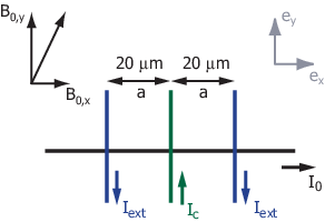
The current in the central wire and the homogeneous field create a two dimensional quadrupole field which strongly confines the atoms in the -plane. Each of the crossing wires contributes a longitudinal field modulation of Lorentzian shape (see [13]):


The two currents together with the field component generate two valleys along the longitudinal axis, which do not appear separate if the trap is located far enough from the surface. The current with its direction opposite to the two external currents is used to split the Ioffe-Pritchard potential into two neighboring wells (fig. 3 a). Choosing the parameters as
| (1) | |||||
| (2) | |||||
| (3) | |||||
| (4) | |||||
| (5) |
the trap is located m above the surface, yielding a transversal oscillation frequency of kHz. The parameter determines the shape of the trap, running from 0 for one single well to 1 for separated wells. The point has been chosen such that the two lowest vibrational levels of each well are clearly separated (i.e., the two lowest sets of states are both degenerate). The time-dependence of the system’s Hamiltonian is expressed via the function . In a simple approach, may be chosen to vary linearly in time, but as we will discuss in section III, an optimized function can be found which minimizes vibrational excitations during the splitting (merging) process.
In fig. 3 a, the resulting magnetic field along the longitudinal axis ex is displayed for characteristic values of ; the transverse potential minimum is plotted against the longitudinal position. The plots below show the eigenstates of 87Rb atoms () in this field as they are numerically computed from the Schroedinger equation (eq. (6) below). The corresponding energy eigenvalues, measured relative to the minimum value of the potential, are given in fig. 4.
For , the four lowest levels correspond to the states of a harmonic oscillator with quantum number and oscillation frequency Hz. We use the quantum number to identify the eigenstates as throughout the whole evolution. As the value of is raised, the vibrational levels evolve into symmetric and antisymmetric delocalized states. At , the four lowest levels form two sets of degenerate states, their energy being , , Hz. At each stage, the separation of the transverse levels ( 50 kHz) is much larger than the separation of longitudinal states involved. For this reason, the longitudinal states do not intermingle with the transverse levels, even if the system’s symmetry is slightly disturbed. The quantum dynamics is therefore adequately described by a one-dimensional model.
In order to make the interferometer work properly, the atomic wave function should follow ideally the (time-dependent) eigenstates of the system. If the potential is varied too fast, the evolution is non-adiabatic, i.e. vibrational excitations are generated. For the investigation of these excitations, we will focus on the first half of the interferometer cycle: we use a time-dependent interaction picture to compute the time scale on which the separation process can be lead adiabatically.
The (time-dependent) basis for the computation is found by solving the time-independent Schrödinger equation
| (6) |
with the Hamilton operator
| (7) |
where takes the role of a mere parameter. For the given magnetic field, the eigenfunctions have been computed numerically and are displayed in fig. 3 b.
The natural phase evolution of the eigenstates can be included into the basis and yields the ansatz
| (8) |
The equation of motion for the coefficients is obtained when eq. (8) is inserted in the time-dependent Schrödinger-equation with the Hamiltonian (7)22 2 The time-dependence of and is explicit through the control parameter : etc.:
| (9) | |||||
Given that a single eigenstate is prepared in the beginning, and further assuming that the transition probability into other vibrational states is small, first order perturbation theory can be used to determine the coefficients and the corresponding transition probabilities :
| (10) | |||||
| (11) |
The coupling to higher levels is directly proportional to the rate at which the control parameter is changed. Therefore, if all levels are separated by a minimum energy , the transition amplitudes can be made negligible by choosing an appropriate duration for the process. Conversely, if at certain instants some energy levels degenerate, this will create large transition amplitudes unless the coupling coefficient between these levels vanishes at the points of degeneration. In the trapped atom interferometer presented here, we encounter such degenerate levels. But as the states that degenerate are of opposite symmetry throughout the complete evolution, the coupling coefficient remains zero for all times. Therefore, the excitation probability can be made arbitrarily small by choosing the process duration long enough.
This consideration is confirmed by numerically evaluating expressions (10) and (11) for either of the interferometer levels . In a first approach, the separation parameter has been chosen linear in time . Fig. 5 shows the transition probabilities into the neighboring interferometer levels which contribute largest to all vibrational excitations. The data indicate that the excitation probability is less than 1% if the separation process takes longer than 60 ms.
This is an encouraging result, as it seems experimentally realizable. Moreover, as the time-dependence of the potential can be freely chosen, one can adjust the speed of the separation process in order to further reduce excitations. This is of general interest, because a linear variation of the control parameter ís not necessarily the best choice. Indeed, one wishes to find a method that optimizes the process irrespective of its parametrization.
III Optimization
In this section, we develop a scheme which minimizes vibrational excitations in time-dependent potentials. In a slight variant, this method can equally be used to find an adequate shape for a beam-splitter potential.

In order to optimize the adiabaticity of the separation process we first take a look at the coupling term from eq. (10)
| (12) |
which is proportional to the process speed and to the coupling coefficient .
Intuitively, one can increase the process speed if is small, and decrease it in the opposite case. Furthermore, the process speed should be adapted to the energy difference of the levels involved, being the more increased the further the energy levels lay apart from each other. Last not least, one has to avoid discontinuities in the process speed including the start and the end of the separation. In the following, these intuitive rules will be substantiated into a set of differential equations to yield an optimized process control .
We assume that the process is lead during and that the separation parameter at is . Indeed, we want to fix a shape of the control parameter which does not depend on the process duration. Therefore, we implicitly assume that can be written as
| (13) |
The goal is then to fix some maximum excitation probability and to find an appropriate shape for the function which minimizes fulfilling the condition
| (14) |
If, by some chance, the distance of energy levels is constant throughout the process, the transition amplitude appears as the Fourier transform of :
| (15) | |||||
| (16) |
If, in addition, happens to be constant over the process, the solution of the problem is simple: the shape of the process speed should be chosen such that it produces the least amount of side bands possible in a Fourier transformation. An appropriate shape would e.g. be a Blackman pulse [14]:
| (17) |
which can be directly integrated to yield .
The idea of the Fourier transform can be extended to the more general case. A substitution of the time variable by some new variable can be made in a way that the argument of the exponential in eq. (15) becomes linear in
| (18) |
and that runs from 0 to 1 during the process. The time scale will be part of the optimization result. Equation (15) then assumes the form of a Fourier transform of some new expression 33 3 In the following equations, the index marks the fact that the functional dependence of the parameter is on , not on .:
| (19) | |||||
| (20) |
The expression is a generalized coupling term, acting in the transformed time frame . As above, one can now choose a shape for this coupling term (however, not its amplitude) and will obtain the probability amplitude as its Fourier transform.
After the optimization strategy is chosen, it remains to solve the equations (18) and (20). One might be tempted to deduce the relation from eq. (18) and insert it into eq. (20) to solve directly for . Unfortunately, this results in an intractable problem. Instead, one can take advantage of the substitution already made and first solve for . The relation between and is then established in a second step. This way, the problem is split into two differential equations the first of which gives the amplitude of , and the second of which determines the time scale used in the substitution. These two values determine size and scale of the probability amplitude .
The first differential equation involves the shape of the function that is chosen for the generalized coupling term , and it is a direct consequence of eq. (20):
| (21) |
It is important to note, that although the time is used to shape the coupling term , its amplitude does not correspond to the overall process speed. Instead, the amplitude of has to be adjusted such that the solution matches the boundary conditions , . This can for instance be done by iteratively solving eq. (21) for different amplitudes of .
The second differential equation establishes the relation between and and arises from the substitution of (eq. (18) ), once that has been determined:
| (22) |
Choosing , this equation can be solved numerically, and one finds as the point in time, for which reaches its boundary .
The result for the transition amplitude is now completely described by equation (19), the amplitude of and the time scale resulting from the choice of the pulse shape. The optimized evolution of the control parameter is computed from the concatenation of and :
| (23) |

If this optimization is applied to the trapped atom interferometer, the probability for non-adiabatic excitations can be considerably reduced. Fig. 6 shows the excitation probabilities for a process speed which has been optimized to suppress the transition . With the optimized control, the separation can be done within 30 ms, thus reducing the complete interferometer cycle to 60 ms with an overall excitation probability of less then .
These parameters suggest that an experimental realization of the scheme is indeed feasible. It remains, of course, a difficult task to prepare the atoms in the ground state and to detect the atoms selectively in different vibrational states. However, this seems achievable using Bose-Einstein condensates of low density. Another issue is stability against gradients of magnetic stray fields. In our case, the sensing states of the interferometer lie m apart. During a sensing time of 60 ms, a gradient would lead to an additional dephasing of . A suppression of stray gradients to less than 1 mG/cm would therefore reduce the dephasing to .
IV Conclusion
In conclusion, we have studied a dynamic potential interferometer working with three-dimensionally trapped atoms. We have used a time-dependent interaction picture to describe the quantum state evolution and we have computed probabilities for non-adiabatic transitions into neighboring levels. For a realistic magnetic microtrap we find parameters which suggests an experimental implementation in the near future. Grounding on the theoretical results, we have developed an optimization scheme for the reduction of vibrational excitations that is independent of the system’s parametrization. Applying the optimization to our interferometer potential, we have found a cycle of duration ms with excitation probability less than .
References
- [1] J. Reichel, W. Hänsel, and T. W. Hänsch, Phys. Rev. Lett. 83, 3398 (1999).
- [2] R. Folman, P. Krüger, D. Cassettari, B. Hessmo, T. Maier, and J. Schmiedmayer, Phys. Rev. Lett. 84, 4749 (2000).
- [3] D. Müller, D. Z. Anderson, R. J. Grow, P. D. D. Schwindt, and E. A. Cornell, Phys. Rev. Lett. 83, 5194 (1999).
- [4] N. H. Dekker, C. S. Lee, V. Lorent, J. H. Thywissen, S. P. Smith, M. Drndič, R. M. Westervelt, and M. Prentiss, Phys. Rev. Lett. 84, 1124 (2000).
- [5] D. Müller, E. A. Cornell, M. Prevedelli, P. D. D. Schwindt, A. Zozulya, and D. Z. Anderson, Opt. Lett. 25, 1382 (2000).
- [6] D. Cassettari, B. Hessmo, R. Folman, T. Maier, and J. Schmiedmayer, Phys. Rev. Lett. 85, 5483 (2000).
- [7] W. Hänsel, J. Reichel, P. Hommelhoff, and T. W. Hänsch, Phys. Rev. Lett. 86, 608 (2001).
- [8] E. A. Hinds, C. J. Vale, and M. G. Boshier, Phys. Rev. Lett. 86, 1462 (2001).
- [9] E. Andersson et al., to be published.
- [10] T. Calarco, E. A. Hinds, D. Jaksch, J. Schmiedmayer, J. I. Cirac, and P. Zoller, Phys. Rev. A 61, 022304 (1999).
- [11] C. Henkel, S. Potting, and M. Wilkens, Europhys. Lett. 47, 414 (1999).
- [12] C. Menotti, J.R. Anglin, J.I. Cirac, and P. Zoller, Phys. Rev. A 63, 023601 (2001).
- [13] J. Reichel, W. Hänsel, P. Hommelhoff, and T. W. Hänsch, Appl. Phys. B 72, 81 (2001).
- [14] R. B. Blackman and J. W. Tukey, The Measurement of Power Spectra from the Point of View of Communications Engineering (Dover Publications, New York, 1958).