Delocalization border and onset of chaos in a model of quantum computation
Abstract
We study the properties of spectra and eigenfunctions for a chain of spins (qubits) in an external time-dependent magnetic field, and under the conditions of non-selective excitation (when the amplitude of the magnetic field is large). This model is known as a possible candidate for experimental realization of quantum computation. We present the theory for finding delocalization transition and show that for the interaction between nearest qubits, the transition is very different from that to quantum chaos. We explain this phenomena by showing that in the considered region of parameters our model is close to an integrable one. According to a general opinion, the threshold for the onset of quantum chaos due to the interqubit interaction decreases with an increase of the number of qubits. Contrary to this expectation, for a magnetic field with constant gradient we have found that chaos border does not depend on the number of qubits. We give analytical estimates which explain this effect, together with numerical data supporting our analysis. Random models with long-range interactions are studied as well. In particular, we show that in this case the delocalization and quantum chaos borders coincide.
pacs
PACS numbers: 05.45Pq, 05.45Mt, 03.67LxI Introduction
In recent years much attention has been paid to the idea of quantum computation [1]. The burst of interest to this subject (see, for example, [2, 3, 4] and references therein) is caused by the discovery of fast quantum algorithms for the factorization of integers [5] and for the effective searching of items in a database [6, 7]. These algorithms demonstrate the effectiveness of quantum computers in comparison with the classical ones. Nowadays, there are different projects for the experimental realization of quantum computers, as well as experimental results with few-qubit systems (see [8]) and references therein).
Main theoretical suggestions for the experimental implementation of the quantum computation are based on interacting two-level systems (qubits ). It is clear that one of the most important problems from the viewpoint of the stability of quantum operations, is a destructive role of different kinds of errors. In the first line, one should refer to finite temperature effects and the interaction with an environment [9]. However, even in the case when these effects can be neglected, there are dynamical effects of the interqubit interaction, which may influence a quantum computation. On one hand, the interaction between qubits is necessary for the realization of quantum computation, on the other hand, it may result in a kind of destruction of the coherence in the evolution of a system.
The latter subject of the dynamical decoherence is directly related to the so-called quantum chaos which is nowadays widely discussed in application to atoms, nuclei, quantum dots and other physical systems (see, for example, [10] and references therein). One of the latest developments in the theory of quantum chaos refers to the interaction between Fermi-particles in isolated systems. The core of this approach is the perturbation theory for many-body states, which takes into account a two-body nature of the interaction. Specifically, it was shown [11] that if the two-body random interaction between particles exceeds some critical value, fast transition to chaos occurs in the Hilbert space of many-particle states (see also [12, 13, 14, 15] and reviews [16, 17]).
In dynamical systems such as complex atoms [18], multicharged ions [19], nuclei [20] and spin systems [21, 22] quantum chaos gives rise to a very complicated structure of highly excited states, and to specific correlations in the energy spectra, described by Random Matrix Theory (RMT) (see, for example, [16]). As a result, closed dynamical systems with relatively small number of interacting particles can be well described by a statistical approach, see discussion and references in [23].
Recently, quantum chaos theory has been applied to a simple model of quantum computer [24] chosen in the form of interacting qubits. Numerical data have shown that for a strong enough interaction between qubits the onset of quantum chaos is unavoidable. Although for the critical value for the quantum chaos border was found to be quite large, with an increase of the border decreases as [25, 24]. From the viewpoint of the standard approach for closed systems of interacting particles, the decrease of chaos border with an increase of qubits looks generic. This poses the question of the relevance of quantum chaos to quantum computation [26, 27].
In our recent paper [29] we have studied the errors which appear in the evolution of 1D Ising nuclear spins in rotating magnetic field. This model was suggested for an experimental realization of a quantum computer [30, 31]. The main attention in [29] has been paid to the region of parameters, most suitable for the preparation of an initial many-body state needed for further application of quantum protocol (sequence of time-dependent magnetic pulses in a prescribed algorithm of quantum computation). It was shown that even for a very large interqubit interaction, the errors turn out to be very small, thus demonstrating that the influence of quantum chaos can be neglected.
An analysis of the stationary Hamiltonian describing the system during a single magnetic pulse has been performed in [28]. Specifically, the general approach of quantum chaos theory has been applied, in order to understand the conditions for the onset of quantum chaos. The model we considered assumed that qubits (nuclear spins) are placed in a strong magnetic field with constant gradient along the direction of the spin chain. The gradient of the magnetic field provides a “labeling” of qubits. Namely, each spins has different Larmor frequency, . This allows one to provide a selective addressing to each qubit by applying resonant rf pulses. The main interest was in the influence of the magnetic field on the properties of eigenstates and energy spectra. It was unexpectedly found that the constant gradient magnetic field gives rise to the independence of the critical value on the number of interacting qubits. This striking phenomena has been explained in [28] analytically and confirmed numerically, thus giving a new insight to the problem of quantum chaos in the models of quantum computers.
In this paper we present the full theory which explains the properties of energy spectra and many-body states of the model of Ref. [29], together with numerical data obtained in a broad region of the model parameters. The structure of the paper is as follows. In the next section we describe the model, discuss the region of parameters of our interest, and briefly analyze the structure of the Hamiltonian matrix in the -representation. In Sect. III we study global properties of the energy spectrum, paying main attention to the band structure of the spectrum and to the level spacing distribution for the central energy band.
Section IV is the core of the paper, here both the delocalization border and the condition for the onset of quantum chaos are studied. The consideration has been made by making use of the mean-field representation which is very convenient from the theoretical viewpoint. One of two main goals of this section is that these two borders are very different in the model with nearest interaction between qubits. Another important result is that the delocalization border turns out to be independent of the number of qubits for a gradient magnetic field. Theoretical estimates obtained in this Section serve as a guiding line to treat all numerical data.
In Section V we investigate numerically the structure of eigenstates in the -representation, by relating the data with the theoretical predictions. Section VI is devoted to some modifications of the model, namely, we analyze the influence of randomness in the interqubit interaction. Our main question is how statistical properties of the system depend on the range of the interaction between qubits. Specifically, we study random interaction between all qubits ( -interaction), as well as between four nearest qubits, by comparing the results with those obtained for the model with the interaction between two nearest qubits (-interaction).
General discussion is presented in the last Section VII. One of the problems we discuss here, is the concept of the quasi-integrability of our model for the -interaction. We show that for the region of parameters of our interest, the model is close to the integrable one. This explains why the delocalization and chaos borders do not coincide for the -interaction. We also analyze the role of the magnetic field. In particular, we give analytical estimates which show that for the homogeneous magnetic field the delocalization border has generic -dependence discussed in [24]. On the other hand, for the magnetic field with an increasing gradient, analytical estimates predict that the delocalization border increases with an increase of the number of qubits.
II The model
The model describes a 1-dimensional chain of interacting distinguishable -spins in an external magnetic field. Schematically, these spins (qubits) can be represented as follows,
Here stands for a constant part of magnetic field oriented in the positive -direction, and each qubit occupies one of two single-particle states with the energy (position “up”) or (position “down”). One can see that the total number of many-body states which are generated by this chain (quantum register), is .
The dynamics of this model (quantum computer protocol) is due to a sum of time-dependent rectangular pulses of a circular polarized magnetic field rotating in the -plane. Each of the pulses has own amplitude , frequency , phase , and lasts during the period . Therefore, the total magnetic field during one pulse can be written as follows,[29],
| (1) |
The Hamiltonian of this system has the form,
| (2) |
where the “pulse function” equals only during the -th pulse of the length . The quantities stand for the Ising interaction between two qubits , are the frequencies of spin’s precession in the magnetic field, is the Rabi frequency corresponding to the -th pulse. The operators are defined by the relations , and , the latter being the Pauli matrices.
Below we consider the properties of the system during a single -th pulse. The corresponding Hamiltonian can be written in the coordinate system which rotates around -axes with the frequency . Thus, for the -th pulse, our model can be reduced to the stationary Hamiltonian,
| (3) |
which describes the evolution of the model for .
The regime of quantum computation corresponds to the following range of parameters: , where [29] (the so-called selective excitation). In this regime, each pulse acts selectively on a chosen qubit exciting a resonant transition. The inequality, , provides a separation between resonant and non-resonant transitions for the same selected qubit. The inequality, , provides a separation of transitions for a given qubit from the transitions for neighboring qubits. In this paper we consider another important regime of non-selective excitation which is defined by the conditions, , see details in [29]. This inequality provides the simplest way to prepare a homogeneous superposition of states needed for implementation of both Shor and Grover algorithms.
In what follows we assume, for simplicity, , and put and . Our main interest is in the nearest neighbor interaction (N-interaction) between qubits for two different cases, the dynamical one when all coupling elements are the same, , and the case when all values are random (random model). However, we will also analyze other cases with different kinds of interaction and compare results with those for the -interaction. In contrast to the previously discussed model [24] with homogeneous magnetic field, below we consider the magnetic field which depends on the position of the -th qubit. Therefore, we assume that the spin frequencies are slightly dependent on (with ).
For the dynamical interaction, the Hamiltonian (3) takes the form,
| (4) |
where . In the -representation the Hamiltonian matrix of size is diagonal for . For the off-diagonal matrix elements are for , and . When calculating the matrix elements of the Hamiltonian (4) we have used the standard rules in order to find the action of the operators and on the states and ,
The matrix turns out to be very sparse, and it has quite specific structure (see Fig.1) in the basis which is reordered according to an increase of the number written in the binary representation, (with or , depending on whether a single-particle state of th qubits is the ground state or the excited state). In what follows, we call this representation as the representation.

III Global properties of the energy spectrum
For the further analysis, it is important to understand the global structure of the energy spectrum. In what follows, we concentrate our attention to the case when the magnetic field has a constant gradient along the chain of qubits, with . Other cases will be briefly discussed in Sect. VII.
III.1 Band structure
Without the interaction between qubits, , the energy spectrum of the model (4) consists of bands of finite width for , separated by big gaps of size . In Ref.[29, 28] it was numerically found that the width of the central band decreases with an increase of as . Our analytical estimates show that for even, the bandwidth is given by the relation , (see details in Sect. IV). This dependence also occurs for a relatively weak interaction . However, when the interaction exceeds some critical value , the band widths turn out to be practically independent on , see the data for the central band in Fig. 2.

The bandwidth for the interaction strength larger than the critical value can be also estimated analytically as (see Sect. IV). The correspondence between the analytical estimate and numerical data was found to be quite good. If the band-width is larger than , the first expression for dominates. Contrary, if the band-width defined by the interaction is larger, it determines the actual band-width which is independent of .
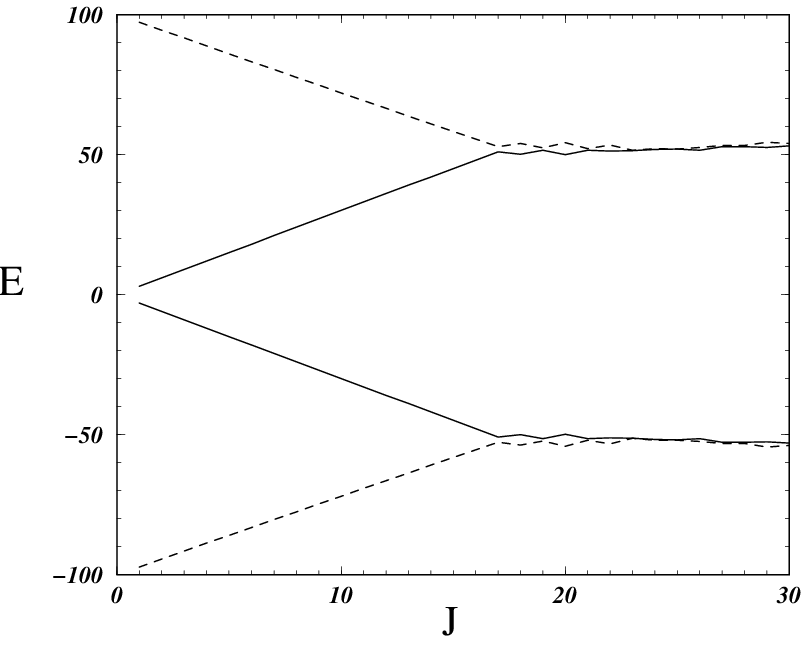
One should stress that the above consideration is valid for the case when the bands are not overlapped. One can expect that for sufficiently strong interaction between the qubits, the band structure of the energy spectrum disappears. The overlapping of the central band with two other bands is shown in Fig.3 where the edges of the central and the nearest bands are plotted in dependence on the interaction for the fixed value . One can see that for the bands are overlapped, therefore, a change in the properties of the system is naturally expected. The critical value for the overlapping of the bands is estimated in Sect. IV as well.
III.2 Level spacing distribution
Let us now analyze the distribution of spacings between nearest-neighbor energy levels inside the central energy band (note that should be normalized to the mean spacing between levels). This quantity is often used in the theory of Quantum Chaos as a detector of chaotic properties of a system. Specifically, for systems with regular motion in the classical limit, the distribution is generically close to the Poisson (apart from 1-dimensional systems where is highly non-generic and can be of any form). In the other limit case of a completely chaotic motion, in the corresponding quantum systems the distribution has the so-called Wigner-Dyson (WD) form which is characterized by the level repulsion for small spacings, (, depending on the symmetry of a system, see, e.g. [16]).
Numerical data for for different values of the interaction strength , summarized in Fig.4, manifest the transition to the WD-distribution. Note that for small values of (see Fig.4a-c) the distribution reveals a strong deviation from the Poisson. Specifically, one can detect a clustering of energy levels for very small , that results in a huge peak in the distribution at the origin . The presence of this peak indicates that for weak interaction our model is highly non-generic and may be compared to integrable 1D-models. With an increase of the interaction, data for reveal, first, a transition to the Poisson, and after, to the WD-distribution. The more detailed analysis of the data shows that the transition from Poisson to WD-distribution occurs when the central energy band starts to overlap with the nearest bands.

IV Theory
Let us now discuss our model (4) from the viewpoint of the standard approach to interacting particles in isolated systems (see, for example, [17, 23] and references therein). In this approach the Hamiltonian is written in the form where stands for non-interacting particles, and describes a two-body interaction between particles. The onset of chaos is usually meant to occur when the strength of the interaction exceeds the mean energy spacing between those many-particle states which are directly coupled by the interaction. It is important to note that this spacing is much larger than the mean level spacing between many-particle states. Indeed, while the total density of states increases exponentially with the total energy, the density increases only algebraically (for details see, e.g., [15]).
In order to apply this approach to our model (4), one needs, first, to present the Hamiltonian as a sum of the “unperturbed” Hamiltonian , and the part that stands for the interaction between particles. In our case the Hamiltonian (4) can be rewritten in the form,
| (5) |
where
| (6) |
As one can see, the Hamiltonian stands for a kind of mean field which absorbs the -dependent term. In this way the “mean field ” describes a regular part of the total Hamiltonian, and the term , describing the interaction between the particles, is responsible for chaotic properties (if any) of the system. Such a mean-field approach is typical in the study of chaotic properties of complex atoms and heavy nuclei [18, 20].
IV.1 Delocalization border
Now, one needs to represent the Hamiltonian (5) in the basis in which it is diagonal in the absence of the interaction (). In this representation (corresponding to the rotating basis) the Hamiltonian can be written as a sum of individual Hamiltonians describing non-interacting quasi-particles [28],
| (7) |
Correspondingly, in the basis of the interaction between quasi-particles has the form, , where
| (8) |
where
| (9) |
From Eq.(7) one can see that the energies of quasi-particles (or, the same, energies of single-particle states determined by the Hamiltonian ) are given by the expression,
| (10) |
Note that this relation is valid for any kind of magnetic field (any dependence ), including the homogeneous magnetic field ().
Let us now consider the constant gradient magnetic field () for large values of . In this case, one can write an approximate relation for ,
| (11) |
This expression allows one to find global properties of the unperturbed () energy spectrum, briefly discussed in the previous section. Indeed, for large values of (more correctly, for ) one can see that the spectrum has a band structure, with the bands centered at .
The central band is defined by such locations of quasi-particles in the single-particle spectra defined by , for which an equal number of quasi-particles have positive and negative values of (for an even number of qubits). Therefore, the total number of many-body states in the central band is given by the total number of combinations of objects having half positive and half negative values,
| (12) |
One can also see that for and , the size of the central energy band is given by twice the maximum energy inside the band,
| (13) |
Now, let us discuss the structure of the Hamiltonian matrix determined by the off-diagonal terms (8). One can see that in the unperturbed basis the term is clearly diagonal. The action of , is much more complicated. Let us consider, for simplicity, the central band. Each operator flips the k-th spin. Since the interaction is two-body, we should consider the action of upon states as , , ,. First two kinds of the states upon the action of still remains in the same central band since the number of ’s and ’s is conserved. Second pair of states increases (or decreases respectively) the number of ’s of two units: that means that such a coupling refers to a next to nearest energy band (nearest bands differ by plus/minus one ’s). As a result, one can conclude that the term stands for the interaction both inside the central band, and between the next-neighbor energy bands.
In the same way it is easy to understand that the term give rise only to the off-band interaction, to be more precise, to a coupling between nearest bands. The structure of the Hamiltonian in the mean-field basis is shown in Fig.5.
For a relatively weak interaction, the eigenstates in the mean-field basis defined by the unperturbed Hamiltonian , are delta-like functions with an admixture of other components with small amplitudes. In this case one can speak about the localization of eigenstates in the unperturbed basis. With an increase of the interaction strength, the number of basis components with large amplitudes (number of principal components) increases. According to the theory of interacting particles, the transition from strongly localized () to delocalized (or, extended) states (with ) occurs very fast with an increase of the interparticle interaction. For this reason, one speaks about the delocalization transition (in the finite-size basis), see, e.g.[14] and references therein.

Generically, in the models with two-body random interaction between particles [15], extended eigenstates with large turn out to be chaotic. By this term we mean the situation when the components of the extended states can be treated as random and independent quantities. Similar situation (the onset of quantum chaos) occurs in many dynamical systems with complex enough interaction, such as many-electron atoms and heavy nuclei [18, 20]. In these systems, the delocalization transition coincides with the transition to chaos, and is determined by the condition (with as a typical interaction strength, and as the mean energy distance between directly coupled many-body states).
Let us now discuss the delocalization transition in our model, keeping in mind that it can be different from the transition to chaos. As it will be shown, our model with the -interaction manifests a quite unexpected phenomena, namely, the above two transitions turn out to be very different.
We start with the estimate of the mean level spacing in the central energy band of our model (5), between the many-body states coupled by the interaction (8). The energy spacing can be estimated as the ratio
| (14) |
where is the number of many-body states coupled by inside the energy interval . In fact, is the mean number per line of non-zero off-diagonal elements in the total Hamiltonian (5).
In order to estimate , we note that the interaction in the central band can only couple those many-body states having an equal number () of spins “up” and “down” (for an even number of qubits). The minimal value of corresponds to the state
and the maximal one, , corresponds to the state
Indeed, in the first case there is only one possibility to change to , and to for the nearest qubits. And in the second case, there are such changes, each of them corresponding to the nearest neighbor interaction with no change in the total number of spins “up” and “down”. Therefore, one can estimate the average value as which is in a very good agreement with direct numerical check.
One should stress that the energy range within which the many-body states are coupled, is much less than the total energy width of the central band determined by Eq.(13). The value of can be estimated as the maximal difference between energies and of two many-body states and of , having the matrix element different from zero. If we consider only the coupling inside the central band we can find these values and by observing that the maximal energy is obtained by flipping the outermost spins. Application of to the state
gives rise to the state
( and correspond to the states with the highest values of single-particle energies ). Thus, the energy difference is given by
Numerical results confirm this prediction very well, see Fig.6.

As a result, for we have,
| (15) |
The mean spacing should be now compared with the typical value of the perturbation, . The latter can be found from as (other terms are negligible for ). Therefore, we finally obtain,
| (16) |
Surprisingly, the delocalization border does not depend on the number of qubits, in contrast to the result of [24] where decreases as . The reason is the specific influence of a constant gradient of the magnetic field that results in the quadratic dependence for the single-particle levels of quasi-particles of the mean-field Hamiltonian (see Eq.(7)).
Let us now compare the analytical estimate (16) with numerical data. The commonly used quantity to measure the number of principal components in eigenstates, is the so-called inverse participation ratio,
| (17) |
Here is the component of a particular eigenfunction corresponding to the eigenvalue .
From Eq.(17) one can see that for equal values of the components of an eigenstate, , the number of principal components is equal to the size of the basis, . In another extreme limit of completely extended and chaotic eigenstates, the value of is equal to . The factor arises due to the Gaussian fluctuations of which are generic in the case of strong quantum chaos (see, e.g.[16] ). For localized states the value of approximately gives the number of basis states effectively occupied by this eigenstate.

Numerical data for computed in the mean field basis (where is diagonal for , see Eq.(5)) for the eigenstates taken from the central energy band, are given in Fig.7 in dependence on . It is clearly seen that below the delocalization border, , there is a scaling dependence of on and in accordance with the estimate (16). On the other side, for , the value of saturates to its maximal value in correspondence with random matrix predictions (here is the total number of states inside the central energy band, see (12)). The latter correspondence of the maximal value of to is a strong evidence of the quantum chaos in the model for a very large interaction.
IV.2 Chaos border
In this section we study the transition to global chaos which is due to the overlapping of the energy bands. In order to obtain the condition for the band overlapping, one needs to find the band width and to compare it with the distance between the bands.
We have shown that in the absence of the interaction, the energy width of the central band can be estimated analytically, see Eq.(13). Numerical data reported in Fig.2, show that with an increase of the interaction, the band width saturates to some value which is independent of . Therefore, we can estimate by coming back to the representation of Hamiltonian (4 ) where the -depending term enters in the off-diagonal matrix elements only. By omitting this term, we can write the diagonal part,
| (18) |
where the relations , and are directly taken into account.
In the case of we are interested in, the unperturbed () many-body energy spectrum of (18) is given by a sequence of degenerate levels separated by the spacing . Due to a weak interaction , each set of these degenerate levels spreads and creates the energy bands. In order to find the central energy bandwidth, we should consider the action of the interaction operator
upon the states belonging to the central band The latter assumption is an approximation: in -representation, the central energy band can also contain few states with slightly different numbers of 0’s and 1’s.
The action of each term in the interaction operator leaves the state as it is, multiplying it by a factor depending on the presence of two close and or different and . This results in the shift of the energy from its zero-value in the central band. Two configurations, and , should be considered which correspond to the maximal shift in the “negative” and “positive” directions. In this way we can safely say that such a bandwidth is given by the energy difference . It is easy to see that one has
and
thus giving
| (19) |
By equating two expressions Eq.(13) and (19) we finds the transition point
| (20) |
between the two dependencies for the band width .
One can see that for bands are overlapped if . That gives the critical value for the overlapping,
| (21) |
subject to the condition . By comparing Eqs.(20) and (21), one gets the lower bound compatible with the above two constraints.
On the other side, one can also have the band overlapping whenever , if . Therefore, in this case the overlapping of the bands occurs for any , if the number of qubits is large enough, .
One should stress that overlapping of bands is not a sufficient condition in order to have the delocalization of eigenstates. Indeed, the estimate Eq.(16) for the delocalization border is derived for the central energy band only, therefore, it is not valid when bands are overlapped. Therefore, one needs to start with the expression (14) and estimate for the case when the energy spectrum is not a band-like.
In order to do this, it is convenient to switch to the mean-field representation with the unperturbed Hamiltonian given by Eq.(6 ). The total size of the unperturbed energy spectrum is now defined by the difference between the energies corresponding to the following limiting configurations,
and
But this is not what we need. Indeed, these two many-body states are not coupled by the two-body interaction (8). What we need to find, is the maximal energy change due to the action of the -interaction. To do that we have to consider two states corresponding to the flipping of both the two uppermost spins, namely :
and
The energy difference between such states is given by :
Since the number of coupled states remains the same, , one gets that in order to have the transition to delocalized states in the case of the overlapped bands, the typical value of the interaction has to be larger than ,
or
| (22) |
One should notice that the two criteria (band overlapping and transition to delocalization), if both satisfied, are expected to result in the onset of chaos. This conclusion is confirmed numerically, and is supported by analytical arguments.
Indeed using data from Fig.4, e.g , , , one gets a chaos border well confirmed by the Wigner-Dyson distribution in Fig.4f.
On the other hand, we have already seen that the simple requirement to be in the delocalized regime without the overlapping of bands, does not give rise to chaos in our dynamical model with the nearest interaction.
It is also easy to check that the conditions of the band overlapping for the case and (with ), are not compatible with the delocalization border in the region of non-selective excitation, . This means that a relatively weak interaction does not lead to the delocalization (and, therefore, to the chaos), in spite of the overlapping of the energy bands.
V Structure of eigenstates in the -representation
The analytical treatment we have performed in the previous section, is based on the mean-field representation of our model, namely, when the Hamiltonian matrix is written in the basis of the “unperturbed” part , see Eq.(7). This approach is natural for the theoretical study since the interaction is much less that the -dependent term (), therefore, the interaction between qubits can be considered as a weak perturbation.
However, the dynamical properties of the model are related to the -representation which is adequate to the experimental setup. For this reason we discuss below the structure of eigenstates of Hamiltonian (4 ) in -representation, in relation with the above analytical estimates obtained in the mean-field approach.
Since the most important question is about the role of the interqubit interaction, main attention is paid to the dependence of global properties of eigenstates on the interaction strength . Typical structure of the eigenstates in the -representation is shown in Fig.8 for different values of . First, one should note that in this basis all components of eigenstates in the absence of the interaction, , are very close, in average, to . If the interaction is very weak, the standard perturbation theory is valid, and a kind of fluctuations of the probabilities is expected around the mean value where is the total size of the basis (the total number of many-particle states).
The data show that if the interaction is relatively strong, the components of eigenstates are quite different from the unperturbed values. This region may be very important for quantum computation, and the main problem is to know whether these errors in the components of the eigenfunctions (the deviations from the unperturbed value ) can destroy quantum coherent effects needed for the quantum computation. This problem was addressed in our previous study [29], here we are mainly interested in global properties of eigenstates for a very broad region of the interaction.
The most interesting conclusion which can be drawn from the numerical data for a weak enough interaction (see Fig.8(a-b)), is that the eigenstates turn out to have a regular structure, even if the deviations are relatively large. Indeed, one can see regular global dependence of on the basis number , with some fluctuations around the mean. This fact seems to be directly related to the specific structure of the Hamiltonian matrix presented in Fig.1.

With an increase of the interaction, the regular structure of eigenstates disappears and huge fluctuations of components of eigenstates emerge, see Fig.8(c-e). The structure of these eigenstates is very similar to that known in the physics of disordered systems, when eigenstates “occupy” some fraction of the basis, without noticeable correlations between different components (see for example, [23] and references therein). One can say that these eigenstates are sparse in the sense that the number of principal components of the eigenstates is much less than the total size of the basis. Therefore, there is a strong change in the structure of eigenstates (compare Figs.8(a-b) with Figs.8(c-e)). One can say that the transition from extended regular states to the weakly chaotic states occurs for .
When the interaction between qubits increases further, one can see another transition to strongly chaotic states, see Fig.8(f). The latter are characterized by an ergodic filling of the whole basis, and by strong fluctuations of the components , which are found to be practically random and independent. This situation is well described by RMT (see, e.g.[32]). Therefore, for such strong interaction , chaotic properties of our system are very strong and quantum computation process can be destroyed.
In order to quantitatively characterize the eigenstates, we have computed the number of principal components defined by Eq.(17). Another measure of the spread of an eigenstate in a given basis, is its ”width” determined as
| (23) |
Note, that in contrast to which gives an effective number of large components, and is insensitive to the location of these components, the width does not ”feel” the presence of ”holes” in the sparse eigenstates. The latter fact can be used to distinguish chaotic ergodic states from the sparse ones. Namely, for fully extended but very sparse eigenstates, the value of is of the order of , however, is much less than .

The mean values of and in dependence on the interaction are given in Fig.9. The circles represent the value of and , averaged over the eigenstates from the central energy band. First of all, one should note that the width turns out to be large and independent of the interaction. This means that all eigenstates are extended in the -representation, in spite of a serious difference in their structure, see Fig.8. Contrary, the number of principal components demonstrates two principal transitions in the structure of eigenstates.
Numerical data of Figs.8-9 allows one to distinguish between few different regions of the interaction strength . The first region with a very weak interaction is characterized by the constant value and corresponds to completely extended () eigenstates shown in Fig.9(a-b). In this region the energy spectrum consists of many close quasi-degenerate levels, thus leading to a strong deviation from the Poisson distribution, see Sect.III.

In the second region with , all eigenstates are strongly influenced by the inter-qubit interaction. This region was termed in Ref.[28] the region of weak chaos since the structure of eigenstates looks chaotic (see Fig.8d), however, the level spacing distribution is quite close to the Poisson. From the data, the transition to the weak chaos occurs for and corresponds to the analytical estimate (16) for the delocalization transition in the mean-field basis. The very point is that the critical value given by Eq.(16), in the -representation corresponds to the transition from completely extended states to the weakly chaotic states. One should stress that from the practical point of view the region of weak chaos may be dangerous for quantum computation because of large deviations of eigenstates from the unperturbed ones, see Fig.8(c-d).
Second transition to strong quantum chaos occurs for . By the latter term we denote the situation when the level spacing distribution has the Wigner-Dyson form and fluctuations of components are close to Gaussian ones with , see Fig.9. As we already discussed, this transition corresponds to the simultaneous occurrence of both band overlapping and delocalized states, see (22). One can see that strong quantum chaos for -interaction emerges for an extremely strong interaction and thus it is not relevant for quantum computation.
More detailed information about the global structure of eigenstates can be drawn from Fig.10 where the value of is shown for all eigenstates reordered in increasing energy . In this figure one can see how the band structure of the spectrum manifests itself in the value of . In particular, it is seen that for non-overlapped bands there is a quite strong dependence of on whether the energy of a specific eigenstate is at the center of energy bands or close to the band edges.
One should point out a remarkable difference for the behavior of close to the band edges, compare Fig.10d and Fig.10e. Namely, in the region of parameters of Fig.10d, the highest value of corresponds to the band edges, in contrast to Fig.10e where at the band edges the eigenstates are extremely localized (with a very small value of ). The origin of this difference is not clear, however, it should be noted that the data reported in Fig.10e have already been observed (and explained) in few models of isolated systems with interacting particles (see, for example, [33] and [34]). For those models it was found that for the unperturbed eigenstates which are close to the band edges, the interaction with other basis states is strongly suppressed.
VI Random Models
In the previous Sections we have discussed the dynamical model (4) of interacting qubits. We have seen that in spite of the absence of any randomness in this model, for a very strong interaction both energy spectra and structure of eigenstates reveal chaotic properties which are generic for quantum chaos. In this sense, it is interesting to compare the obtained results with those for similar models with random interaction. This problem is not academic since in reality there are many effects which can lead to some randomness in the Hamiltonian (3).
VI.1 All-to-all interaction
It is instructive to see what happens for a long-range interaction between qubits. We have studied in details the case when the interaction couples all qubits in the same manner (-interaction),
| (24) |
Here the interaction is assumed to be completely random, with where are random numbers with a flat distribution inside the interval .
This model can be treated analytically in the same way as we did it in Sect.IV. Specifically, we are interested in the delocalization border which is determined by the comparison of the ratio (14) with the typical interaction strength.
The modification of the Hamiltonian (5) written in the mean field basis is straightforward. Specifically, the structure of the unperturbed part, see Eq.(7), remains the same, and the interaction term (8) has the same structure (the only difference being the summation taken over all qubits). The most important point is that the Hamiltonian matrix has a different structure from that for the interaction, see Fig.11

Despite the block structure shared by the analogous matrix for the -interaction, shown in Fig.(5), and due to two-body interaction, each block is now characterized by many elements different from zero. For this reason, one can expect that chaotic properties of the model with the -interaction are much stronger that those found in the case of -interaction.
The estimate for can be obtained for the -interaction as well. Since all qubits are allowed to interact to each other, the maximum number of coupling between unperturbed many-body states inside the central energy band with all the others, is
| (25) |
As for , it can be found by considering the maximal energy shift obtained by applying the operator to the state and resulting in the new state The energy difference between these two states is given by
which perfectly agrees with the direct computations, see Fig.6. As a result, the critical value for the delocalization border is obtained from the relation,
therefore,
| (26) |

This is an unexpected result since it coincides with the estimate (16) for the delocalization border in the case of -interaction. The reason is that the energy range within which many-body states are connected by the interaction, and the number of the states within this energy range, are both proportional to . The result shows that the delocalization border turns out to be independent on the range of the interqubit interaction.
However, chaotic properties of this random model with the -interaction are much stronger than those found for the -interaction. Namely, the chaos border for the -interaction turns out to coincide with the delocalization border. The transition to delocalized states for the interaction is shown in Fig.12.
The closeness of the delocalization and chaos borders for the -interaction can be also checked by studying the level spacing distribution. The latter is expected to manifest a transition from the Poisson to the Wigner-Dyson at the critical value of given by the above estimate (26). In Fig.13 we show that the transition to chaos is independent from the product , in correspondence with the analytical prediction (26). These results prove that for the -interaction our model is similar to generic models for which the delocalization border coincides with the chaos border.

VI.2 Next to nearest interaction
Finally, we discuss the intermediate case when the interaction in the dynamical model (3) couples four next nearest qubits, , (the -interaction).
A straightforward analysis similar to that shown in the previous Sections leads to the same critical border for delocalized states, as those found for the and interactions. This has been numerically confirmed, see that data in Fig.12. Moreover, as for the -interaction, the delocalization border for the -interaction turns out to coincide with the chaos border. This has been proved by using the level spacing distribution, see Fig.14.
Our numerical study shows that, in contrast to the case of the -interaction (when only two neighbor qubits are coupled), the quantum chaos emerges for much lower values of the -interaction, for , see Figs.14. This region of parameters and is important from the experimental viewpoint, therefore, the quantum chaos may have a real influence for quantum computation.

Since any other of long range interactions can be seen within these two extreme cases (the and interactions), one can conclude that for a typical interaction (other than strictly between nearest qubits), the quantum chaos can emerge for a quite weak interaction and may have an influence on a quantum computer operability. Therefore, it may be important to reduce the range of the interqubit interaction in an experimental setup of a quantum computer.
VII General discussion
VII.1 Quasi-integrability
As we noted, the model (4) with the interaction between nearest qubits has quite specific properties. Namely, the delocalization border turns out to be very different from the border of quantum chaos. Below we explain this phenomena in terms of quasi-integrability of our model.
Let us come back to the expression for the off-diagonal matrix elements of the Hamiltonian (5) in the mean-field basis determined by the eigenstates of , see Eqs.(8). For the case of large , we are interested in, the term is small compared to since and . Also, the diagonal term is much smaller than the two other terms (it is proportional to , see Eq.(9)). Therefore, the approximate Hamiltonian can be written in the following form
| (27) |
where and for our model.
This Hamiltonian has been recently studied in a number of papers, (see, for example, [35] and references therein). It was shown [36] that for independent random variables and the model (27) can be mapped to an Hamiltonian describing free fermions. This transformation holds only in the case of nearest neighbor coupling. Therefore, this model is integrable and the level spacing distribution can be expected to be Poisson–like for any interaction strength . This explains why for non-overlapping bands our original Hamiltonian (6) with reveals the Poisson for above the delocalization border.
It should be noted that the delocalization border (see Sect.IV) results from the standard perturbation theory which takes into account a two-body nature of interaction. Namely, when the typical interaction which connects unperturbed many-body states is much larger than the mean distance between energy levels of these states, in the corresponding basis the interaction creates exact eigenstates with many components. Typically, these compound states are chaotic due to a complex structure of the interaction. This is why the delocalization border generically coincides with the quantum chaos border. However, in specific cases like our quasi-integrable model (for and not very strong interaction), the delocalization border and the onset of chaos may be very different.
The above analysis is also helpful in the explanation of the strong difference between the model with -interaction, from the model when qubits are coupled by a different kind of interaction ( or interaction, see previous Sections). Indeed, in the latter cases the interaction has many additional terms compared with Eq.(8), and results in a strong coupling between all energy bands. This leads to quasi-integrability breaking, and to the onset of chaos at the border of delocalization.
VII.2 Role of magnetic field
Our approach based on the mean-field representation, see Sect.IV, is valid for any kind of the -magnetic field. Let us consider the simplest case of a homogeneous magnetic field for which all frequencies of spin’s precession are the same, . For a non-resonant case with , and in absence of the interaction (), the energy spectrum has no more a band structure since each of the levels is degenerate. Indeed, each single-particle energy has two values only, where . Since all many-body states in the central band have the same number of pluses and minuses in the expression for the total energy, the latter is zero. Thus, the level spacing is also zero which means that any small interaction gives rise to delocalized states.

In recent studies [24] random variation of spin frequencies is included in the model, in order to take into account effects of finite temperature and environment. For this reason the energies are not exactly degenerate but swap into finite width bands. In the same way, let us assume that the energy of many-body states fluctuates, thus resulting in the distribution of the parameter within some interval with . Then, one can estimate,
On the other side, the number of coupled state for a fixed state from the central band remains the same, As a result the delocalization border can be determined from the relation,
| (28) |
This parametric dependence has been checked numerically (see Fig.15) where the average number of principal component is plotted against the rescaled interaction for different and . As one can see, the scaling law given by Eq.(28) is quite well satisfied. Comparing with Fig.9, one should note that for a constant magnetic field the onset of a strong chaos () happens in a very small region of interaction (see the presence of small peaks on the far right side). With further increase of the interaction, the system again becomes nearly-integrable, since in the limit only diagonal terms dominate.
In this way we come to the same -dependence for the critical interaction , discussed in Refs.[25, 24]. In these papers, the model with a nearest interaction in the plane was considered (rather than on 1D line as in our model). For this reason the model of Refs.[24] is free from the effects of quasi-integrability and, therefore, the delocalization border coincides with the border of quantum chaos.
Finally, we would like to point out that in the case of increasing gradient of the -magnetic field, the delocalization border increases with an increase of the number of qubits. This very unexpected prediction can be easily understood for the case (linear increase of the gradient). It can be shown that the width grows proportional to , therefore, for the nearest interaction () the critical interaction increases as , and for the -interaction one gets, . In the latter case the estimate of also gives the transition to the chaos. As one can see, the magnetic field with an increasing gradient may strongly reduce the influence of the delocalization and chaos.
VIII Acknowledgments
The work of GPB and VIT was supported by the Department of Energy (DOE) under the contract W-7405-ENG-36, by the National Security Agency (NSA) and Advanced Research and Development Activity (ARDA). FMI acknowledges the support by CONACyT (Mexico) Grant No. 34668-E
References
- [1] R.P. Feynman, Found. Phys. 16, 507 (1986); Feynman Lectures on Computation, Perseus Books, 1996.
- [2] A. Steane, Rep. Progr. Phys., 61, 117 (1998).
- [3] G.P. Berman, G.D. Doolen, R. Mainieri, and V.I. Tsifrinovich, Introduction to Quantum Computers, World Scientific Publishing Company, 1998.
- [4] M.A. Nielsen, I.L. Chuang, Quantum Computation and Quantum Information, Cambridge University Press, 2000.
- [5] P. Shor, Proc. of the 35th Annual Symposium on the Fundations of Computer Science, IEEE, Computer Society Press, New York, (1994), p.124.
- [6] L.K. Grover, Phys. Rev. Lett., 79, 325 (1997); ibid. 80, 4329 (1998).
- [7] I.L. Chuang, N.A. Gershefeld, M. Kubinec, Phys. Rev. Lett., 80 (1998) 3408.
- [8] G.P. Berman, G.D. Doolen, V.I. Tsifrinovich, Superlattices and microstructures, 27 (2000) 89.
- [9] I.L. Chuang, R. Laflamme, P.W. Shor, and W.H. Zurek, Science, 270, 1633 (1995)
- [10] New Directions in Quantum Chaos, Proceedings of the International School of Physics ”Enrico Fermi”, Course CXLIII, Varenna 20-30 July, eds. G.Casati, I.Guarneri and U.Smilansky, IOS Press, 2000.
- [11] B.L. Altshuler, Y. Gefen, A. Kamenev and L.S. Levitov, Phys. Rev. Lett., 78, 2803 (1997).
- [12] S. Aberg. Phys. Rev. Lett. 64, 3119 (1990).
- [13] V.V.Flambaum, F.M.Izrailev, and G.Casati, Phys. Rev. E 54, 2136 (1996); V.V. Flambaum and F.M.Izrailev, Phys. Rev. E 55, R13 (1997).
- [14] V.V. Flambaum and F.M. Izrailev, Phys. Rev. E 56, 5144 (1997).
- [15] V. V. Flambaum and G. F. Gribakin, Phys. Rev. C 50, 3122 (1994); D. L. Shepelyansky and O. P. Sushkov, Europhys. Lett. 37, 121 (1997); A. D. Mirlin and Y. V. Fyodorov, Phys. Rev. B 56, 13393 (1997); D. Weinmann, J. -L. Pichard and Y. Imry, J.Phys. I France, 7, 1559 (1997); P. Jacquod and D. L. Shepelyansky, Phys. Rev. Lett. 79 , 1837 (1997); P. G. Silvestrov, Phys. Rev. Lett., 79, 3994 (1997); Phys. Rev. E. 58, 5629 (1998).
- [16] T. Guhr, A. Müller-Groeling, and H.A. Weidenml̈ler, Phys. Rep., 200, 189 (1999).
- [17] F.M. Izrailev, in Ref.[10], pp.371-430.
- [18] V. V. Flambaum, A. A. Gribakina, G. F. Gribakin, and M. G. Kozlov, Phys. Rev. A 50, 267 (1994).
- [19] G.F. Gribakin, A.A. Gribakina, V.V. Flambaum. Aust.J.Phys. 52, 443 (1999).
- [20] M.Horoi, V.Zelevinsky and B.A.Brown, Phys. Rev. Lett. 74, 5194 (1995); V.Zelevinsky, M.Horoi and B.A.Brown, Phys. Lett. B 350, 141 (1995); N.Frazier, B.A.Brown and V.Zelevinsky, Phys. Rev. C 54, 1665 (1996); V.Zelevinsky, B.A.Brown, M. Horoi and N.Frazier, Phys. Rep., 276 , 85 (1996).
- [21] V. V. Flambaum, Proc. 85th Nobel Symposium, Phys. Scr. 46, 198 (1993).
- [22] B. Georgeot and D. L. Shepelyansky, Phys. Rev. Lett. 81,5129 (1998).
- [23] F.M.Izrailev, to be published in the Proceedings of the Nobel Simposia “Quantum Chaos Y2K”, Physica Scripta, 2001; cond-mat/0009207.
- [24] B. Georgeot and D.L. Shepelyansky, Phys. Rev. E., 62, 3504 (2000); ibid, 6366.
- [25] B. Georgeot and D. Shepelyansky, Phys. Rev. Lett., 81, 5129 (1998).
- [26] V.V. Flambaum. Aust.J.Phys. 53, N4, (2000).
- [27] P.G. Silvestrov, H. Schomeraus, and C.W.J. Beenakker, quant-ph/0012119.
- [28] G.P. Berman, F. Borgonovi, F.M. Izrailev, and V.I. Tsifrinovich, quant-ph/0012106.
- [29] G.P. Berman, F. Borgonovi, F.M. Izrailev, and V.I. Tsifrinovich, quant-ph/0006095.
- [30] G.P. Berman, G.D. Doolen, G.D. Holm, V.I. Tsifrinovich, Phys. Lett. A , 193 (19 94) 444.
- [31] G.P. Berman, G.D. Doolen, V.I. Tsifrinovich, Computer Physics Communications, 127 (2000) 91.
- [32] F.M. Izrailev, Phys.Rep. 196, 299 (1990).
- [33] F. Borgonovi, I. Guarneri and F.M. Izrailev, Phys. Rev. E. 57, 5291 (1998).
- [34] G. A. Luna-Acosta, J. A. Méndes-Bermúdez, and F. M. Izrailev, Phys. Lett. A., 274, (2000) 192.
- [35] A.P. Young and H. Rieger, Phys. Rev. B, 53, 8486 (1996); A.P. Young, Phys. Rev. B, 56, 11691 (1997).
- [36] E. Lieb, T. Schultz,and D. Mattis, Ann. Phys. (N.Y.) 16, 407 (1961).