Robust quantum memory via quantum control

© 2026 Optical Society of America
OCIS codes: 270.0270, 270.1670

Quantum computation [1] has been a fruitful area of research lately. Some of the most promising schemes involve encoding qubits into ions and neutral atoms in high Q optical cavities. One of the greatest limitations to such schemes is the decoherence which occurs at the optical transitions. This decoherence is the limiting factor in determining the temporal length of a sequence of pulses to perform a given computation. Many schemes have been suggested to overcome this decoherence, especially quantum error correction [2], which uses redundant information to compensate for the losses, and decoherence-free substates [3], which use combinations of states which are robust against decay because of quantum interference. In this paper we employ Lie group decompositions [4] to derive a promising scheme for a quantum memory, with the idea being to transfer quantum information from the important channel for quantum information processing to a “memory transition” which holds the quantum information.

Our scheme can be illustrated with a simple example. Consider a four-level atom as depicted in figure 2 with two degenerate ground states $|g_{1}\rangle$ and $|g_{2}\rangle$ and two non-degenerate excited states $|e_{1}\rangle$ and $|e_{2}\rangle$. The ground states might be for example Zeeman sublevels of an atom such as Rubidium, although our scheme is far more general than this. We assume that the $|g_{1}\rangle-|e_{1}\rangle$ transition is an optical transition that forms part of a quantum information processing scheme. After performing some quantum logical operations we wish to protect the quantum information stored in this transition in a long-lived system by applying a series of Gaussian control pulses (derived from optical fields) to transfer the quantum information onto the decoherence-free $|g_{1}\rangle-|g_{2}\rangle$ transition. Although the transition pairs $|g_{1}\rangle-|e_{1}\rangle$, $|g_{2}\rangle-|e_{1}\rangle$ and $|g_{1}\rangle-|e_{2}\rangle$, $|g_{2}\rangle-|e_{2}\rangle$ are at equal frequencies, they can be individually addressed through the choice of appropriate field polarisations, allowing complete controllability of the system.

Formally, the problem can be stated as follows. We wish to map the density matrix $\rho$ representing the (initial) state of the system, whose elements are $\rho_{g_{1}g_{1}}$, $\rho_{e_{1}e_{1}}$, $\rho_{g_{1}e_{1}}$ and $\rho_{g_{2}g_{2}}=\rho_{e_{2}e_{2}}=\rho_{g_{1}g_{2}}=\rho_{g_{1}e_{2}}=\rho_{g_{2}e_{1}}=\rho_{g_{2}e_{2}}=0$, onto a density matrix $\rho^{\prime}$ such that $\rho_{g_{1}g_{1}}^{\prime}=\rho_{g_{1}g_{1}}$, $\rho_{g_{2}g_{2}}^{\prime}=\rho_{e_{1}e_{1}}$, $\rho_{g_{1}g_{2}}^{\prime}=\rho_{g_{1}e_{1}}$ and $\rho_{e_{1}e_{1}}=\rho_{e_{2}e_{2}}=\rho_{g_{1}e_{1}}=\rho_{g_{1}e_{2}}=\rho_{g_{2}e_{1}}=\rho_{g_{2}e_{2}}=0$ by applying a sequence of simple control pulses. Because the populations and coherence have been mapped to degenerate energy levels with no allowed transitions between them, these states will be extremely long lived. The quantum information can then be returned to the optical transition simply by using the reverse of the quantum control scheme. In order to realize the mapping of $\rho$ onto $\rho^{\prime}$ we find a unitary operator $U$ such that $\rho^{\prime}=U\rho U^{\dagger}$ and decompose the operator $U$ into a product of simple unitary operators, each realized dynamically by applying a control field 1 (2) (3) that drives the $|g_{2}\rangle-|e_{2}\rangle$ ($|g_{1}\rangle-|e_{2}\rangle$) ($|g_{1}\rangle-|e_{1}\rangle$) transition, respectively. Concretely, note that we have

Furthermore, we can express $U$ as a product $U=V_{1}V_{2}V_{3}V_{2}V_{1}$ where

Observing that [4]

we see that the operator $V_{1}$ can be dynamically realized by applying a pulse $f_{1}(t)=A_{1}(t)e^{i\omega_{g_{2}e_{2}}+\pi/2}$ with total pulse area $\int|A_{1}(t)|\,dt=\pi/(2d_{g_{2}e_{2}})$ and appropriate polarisation, where $\omega_{g_{2}e_{2}}$ is the frequency and $d_{g_{2}e_{2}}$ the absorption oscillator strength of the $|g_{2}\rangle-|e_{2}\rangle$ transition. Similarly,

shows that $V_{2}$ [$V_{3}$] can be dynamically realized by applying a pulse $f_{2}(t)=A_{2}(t)e^{i\omega_{g_{1}e_{2}}+\pi/2}$ [$f_{3}(t)=A_{3}(t)e^{i\omega_{g_{1}e_{1}}+\pi/2}$] with appropriate polarisation and total pulse area $\int|A_{2}(t)|\,dt=\pi/(2d_{g_{1}e_{2}})$ [$\int|A_{3}(t)|\,dt=\pi/(2d_{g_{1}e_{1}})$] where $\omega_{g_{1}e_{2}}$ [$\omega_{g_{1}e_{1}}$] is the frequency and $d_{g_{1}e_{2}}$ [$d_{g_{1}e_{1}}$] the absorption oscillator strength of the $|g_{1}\rangle-|e_{2}\rangle$ [$|g_{1}\rangle-|e_{1}\rangle$] transition.

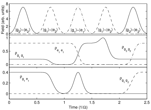
Hence, generation of $U$ requires a sequence of five pulses, where the first pulse drives the transition $|g_{2}\rangle-|e_{2}\rangle$ and has pulse area $\pi/(2d_{g_{2}e_{2}})$; the second pulse drives the transition $|g_{1}\rangle-|e_{2}\rangle$ and has pulse area $\pi/(2d_{g_{1}e_{2}})$; the third pulse drives the transition $|g_{1}\rangle-|e_{1}\rangle$ and has pulse area $\pi/(2d_{g_{1}e_{1}})$; the fourth pulses drives again the transition $|g_{1}\rangle-|e_{2}\rangle$ and has pulse area $\pi/(2d_{g_{1}e_{2}})$ and the last pulse drives again the transition $|g_{2}\rangle-|e_{2}\rangle$ and has pulse area $\pi/(2d_{g_{2}e_{2}})$. Observe that only the total area of each pulse matters and hence the precise pulse envelopes can be adjusted to suit experimental constraints.

Figure 2 shows the pulse sequence and evolution of a system initially in the superposition state $(|g_{1}\rangle+2|e_{1}\rangle)/\sqrt{5}$. Note that initially $\rho_{g_{1}g_{1}}=0.2$, $\rho_{e_{1}e_{1}}=0.8$, $\rho_{g_{1}e_{1}}=0.4$ and all other matrix elements of $\rho$ are zero. Observe that at the final time we have indeed $\rho_{g_{1}g_{1}}^{\prime}=0.2$, $\rho_{g_{2}g_{2}}^{\prime}=0.8$, $\rho_{g_{1}g_{2}}=0.4$ and all other elements of $\rho^{\prime}$ are zero. The time unit in all plots is $1/\Omega$, where $\Omega$ is the Rabi frequency of the transition $|g_{1}\rangle-|e_{1}\rangle$.

One of the authors (ADG) would like to acknowledge the financial support of the EPSRC.

References

- [1] M. A. Nielsen and I. L. Chuang, Quantum Computation and Quantum Information (Cambridge University Press, 2000)
- [2] D. Gottesman, “An introduction to quantum error correction,” http://xxx.lanl.gov/abs/quant-ph/0004072
- [3] A. Beige et.al, Phys. Rev. Lett 85, 1762 (2000); D. A. Lidar et.al, Phys. Rev. A 63, 022307 (2001)
- [4] V. Ramakrishna et.al., Phys. Rev. A 61, 032106 (2000)
Abstract
A general scheme for building a quantum memory by transferring quantum information to an essentially decoherence-free memory transition using quantum control is presented and illustrated by computer simulations.