The asymptotic relative entropy of entanglement

The systematic investigation of quantum entanglement is a major goal of quantum information theory [1]. In the study of entanglement manipulation one considers the interconversion of different forms of entanglement by means of local quantum operations and classical communication (LQCC). For pure bi-partite states entanglement manipulation in both the finite and asymptotic limits is quite well understood. For pure states necessary and sufficient conditions for the local interconvertibility of entangled states are known. In the asymptotic limit of infinitely many copies of a pure state, a single number, the von Neumann entropy of a subsystem, appropriately quantifies the degree of entanglement [2].

Much less is known about the entanglement of mixed states. One approach is to define entanglement measures, which are functions of a state that cannot increase under local operations and provide constraints on possible local entanglement manipulation protocols. These measures prove to be useful mathematical and conceptual tools, and have interesting links with other areas such as the study of channel capacities [3]. A number of such measures have been proposed, most notably the entanglement of formation [3], the distillable entanglement [3, 4], and the relative entropy of entanglement [4, 5]. The distillable entanglement is defined as the asymptotic number of pure maximally entangled states that can be obtained via LQCC from a supply of a given state. For mixed states the distillable entanglement is exceedingly difficult to compute as it is defined as an asymptotic quantity referring to infinitely many copies of a quantum state. Therefore, upper bounds on the distillable entanglement, in particular other entanglement measures, are of major practical use. One such entanglement measure is the relative entropy of entanglement, defined as

for states $\sigma$, where ${\cal D}$ is the set of states with positive partial transpose (PPT states), and $S(\sigma||\rho)=\text{tr}[\sigma\lg\sigma-\sigma\lg\rho]$ ($\lg$ signifies $\log_{2}$). This function essentially quantifies the distinguishability of $\sigma$ from the set of PPT states. The set ${\cal D}$ can also be taken to be the set of separable states [5]. However, the set of PPT states is much easier to characterise, and the resulting measure provides a tighter bound to the distillable entanglement, one that is actually attained on pure states and certain mixed states [3].

In general, efficient protocols for entanglement manipulation require an asymptotic number of copies of the initial state. Therefore, to address any question related to asymptotic entanglement manipulation, one will instead have to consider asymptotic versions of the entanglement measures. For a given measure of entanglement $E$, the asymptotic version $E^{\infty}$ is defined as the average entanglement per copy in the asymptotic limit [6, 7],

For example, the asymptotic cost of creating a mixed state by LQCC from a supply of pure maximally entangled states is given by the asymptotic entanglement of formation [7]. However, such asymptotic entanglement measures are difficult to compute, and so far this task has not been accomplished except for the very rare occasions where the measure in question is known to be additive[8].

In this Letter we present a general formula for the asymptotic relative entropy of entanglement for an important class of bi-partite states, namely the Werner states of arbitrary dimension [9]. These states are the only states that are invariant under local unitaries of the form $U\otimes U$. They can be conveniently formulated in terms of the projectors $\pi_{0}$ ($\pi_{1}$) on the symmetric (antisymmetric) subspaces of a Hilbert space ${\cal H}={\mathbb{C}}^{d}\otimes{\mathbb{C}}^{d}$. Denoting the permutation operator that interchanges the subsystems as $\pi$, the projectors can be expressed as $\pi_{0}=(\openone+\pi)/2$ and $\pi_{1}=(\openone-\pi)/2$. A general Werner state is of the form $\sigma(p)=p\sigma_{1}+(1-p)\sigma_{0}$, $p\in[0,1]$, where $\sigma_{0}=\pi_{0}/\text{tr}[\pi_{0}]$ and $\sigma_{1}=\pi_{1}/\text{tr}[\pi_{1}]$. Appropriately exploiting the symmetry of this state is one of the key ingredients to the proof of the main statement of this Letter. We formulate this main result as a theorem.
Theorem. For states in ${\mathbb{C}}^{d}\otimes{\mathbb{C}}^{d}$ of the form $\sigma(p)=p\sigma_{1}+(1-p)\sigma_{0}$ with $p\in(1/2,1]$, $E_{R}^{\infty}$ w.r.t. PPT states is given by

where $H(p)=-p\lg p-(1-p)\lg(1-p)$.

It is interesting to note from this formula that $E_{R}^{\infty}$ never exceeds the logarithm of the negativity [10]. Curiously, $E_{R}^{\infty}(\sigma(p))$ is a convex function of $p$, whereas numerics show that $E_{R}(\sigma(p)^{\otimes n})/n$ is not convex for any finite number $n>1$. It is also intriguing that this formula is exactly the same as that from a different optimization problem considered by Rains [11], where he minimizes the function $B(\rho,\sigma)=S(\rho||\sigma)+\log|\sigma^{\Gamma}|$ over all states $\sigma$. Rains’ quantity is also an upper bound to the distillable entanglement. However, it is not a convex function, which makes its minimization difficult due to the possibility of local minima. This applies especially in the asymptotic limit as the additivity properties of $B(\rho,\sigma)$ are unknown.

Proof: The proof proceeds in two stages. First we provide an upper bound on $E_{R}(\sigma^{\otimes n})/n$ for any number of copies $n$, by presenting a trial optimal state. Then we derive a lower bound for $E_{R}(\sigma^{\otimes n})/n$ using convex optimization methods. We conclude by showing that the two bounds coincide in the asymptotic limit $n\rightarrow\infty$.

Upper bound: We consider a situation where we hold $n$ copies of a Werner state $\sigma(p)$. Following the work of Ref. [12], we will make heavy use of symmetry. In Refs. [4, 12] it has been shown that if a state is invariant under a certain symmetry group, then one can restrict the minimization in Eq. (1) to those PPT states that are also invariant under the same group. As $\sigma(p)$ is invariant under the group $G$ of local unitaries of the form $U\otimes U$, the state $\sigma(p)^{\otimes n}$ is invariant under $G^{\otimes n}$. This implies that the optimal PPT state for $\sigma(p)^{\otimes n}$ can be chosen to be a convex sum of the $2^{n}$ possible $n$-fold tensor products of $\sigma_{0}$ and $\sigma_{1}$,

where $\vec{x}=(x_{0},...,x_{2^{n}-1})^{T}$ forms a probability distribution, and $f_{i}\in\{0,1\}$, $i=1,...,n$, is the $i$-th digit in the binary representation of $f$. Furthermore, as the state $\sigma^{\otimes n}$ is invariant under any permutation of the $n$ copies, we can add the constraint that $x_{l}=x_{m}$ if the number of 1’s in the binary representations of $l$ and $m$ are the same.

We will consider trial states of the form $\sum_{i}w_{i}(u_{i}\sigma_{1}+v_{i}\sigma_{0})^{\otimes n}$ , which automatically satisfy this constraint. Such states correspond to:

where the $u_{i}(v_{i})$ component is the weight of $\sigma_{1}(\sigma_{0})$, $u_{i}+v_{i}=1$ and $\sum_{i}w_{i}=1$ (and therefore $\sum_{j}x_{j}=1$).

We will need to know the eigenvalues of the partial transpose of $\eta$ in order to ensure that it is PPT. Ignoring degeneracy, there are only two eigenvalues of the partial transpose of the Werner state $\sigma(p)$. It is easy to show that they are non-negative iff the following two component vector is non-negative:

Similarly, it can easily be shown that $\eta$ will be a PPT state iff the $\vec{y}$ and $\vec{x}$ in the following equation are non-negative vectors:

Subject to this condition we need to calculate the relative entropy between the $n$-copy Werner state $\sigma(p)^{\otimes n}$ and this generalized Werner state $\eta$. This is given by:

At this point, we notice that since the second term in Eq. (11) is the average of the function

over a binomially distributed variable $k$, the value can be substituted by $\xi(np)$ when we take the limit $n\rightarrow\infty$ [13].

Since $E^{\infty}_{R}(\sigma(p))$ is the minimal value of $S(\sigma(p)^{\otimes n}||\eta)/n$ over all possible PPT states $\eta$, any such PPT state $\eta$ will give us an upper bound for $E_{R}^{\infty}(\sigma(p))$. In particular, for the vector $\vec{x}$ we propose a mixture of two $n$-fold Kronecker powers:

where $0\leq w_{i}\leq 1$, $w_{1}=1-w_{2}$, $0\leq a_{1}\leq 1/2$ and $1/2\leq a_{2}\leq 1$. Proper values for the parameters need to be selected, to ensure that the corresponding state $\eta$ will be PPT. Inspired by numerical results, we consider two separate intervals for $p$ in Eq. (The asymptotic relative entropy of entanglement); $1/2\leq p\leq(d+2)/(2d)$, and $(d+2)/(2d)\leq p\leq 1$.

For the first interval, set $w_{1}=0$ and $a_{2}=1/2$, so that $x_{k}=2^{-n}$ for all $k$. This state gives us an upper bound that equals $E_{R}$ for one copy of $\sigma(p)$

Now consider the second interval. We will set

We calculate $T^{\otimes n}\vec{x}$:

so that, with the values of Eq. (The asymptotic relative entropy of entanglement)

where $\#(k)$ is the number of 1’s in the binary representation of $k$. It is easy to check using Eq. (The asymptotic relative entropy of entanglement) that $y_{k}$ is always non-negative.

As a consequence, by taking into account the discussion after Eq. (11) and the notation introduced in Eq. (8), the upper bound for $n\rightarrow\infty$ reads

with

It is easy to check that for $p\geq(d+2)/(2d)$ (the second interval), both $t_{1}\geq t_{2}$ and $q_{1}\geq q_{2}$. So we obtain:

In the other regime, $p\leq(d+2)/(2d)$, the bound obtainable from Eq. (20) is worse than Eq. (14). This ends the proof of the upper bound.

Proof of lower bound: We now proceed to find a lower bound on $E_{R}$. To do this, we will use the idea of Lagrange duality [14]. To calculate $E_{R}^{\infty}$ we need to solve the optimization problem

where $\vec{z}^{T}=(p,1-p)^{\otimes n}$. This is a convex optimization problem, so it is possible to consider the so-called dual problem. It is a basic result in convex optimization theory that the optimal (maximal) $g$-value of the dual problem is a lower bound on the optimal (minimal) value of the primal problem, which is just what we are looking for (see [14] for a general description of duality in optimization).

The dual problem can be obtained as follows. First form the Lagrangian by multiplying the constraints with Lagrange multipliers and adding them to the objective function:

The constraint $\vec{x}\geq 0$ is not included explicitly, as it just determines the domain of the function $\lg$. Note that $\vec{\lambda}$ must exhibit the same copy-permutation symmetry as $\vec{x}$. Because the constraint associated to $\vec{\lambda}$ is an inequality, we have to introduce the constraint $\vec{\lambda}\geq 0$. The dual function is now given by

and the dual optimization problem is:

including any other constraints on the domain of $g$.

For our problem, the dual function can be calculated explicitly. The derivative of the Lagrangian w.r.t. $x_{k}$ is

The Lagrangian reaches an extremum (minimum) at

where $\mu_{k}=\nu-\left(T^{\otimes n}\vec{\lambda}\right)_{k}$ and we have exploited the symmetry of $T$. The dual function is

where we have used that $\vec{z}^{T}=(p,1-p)^{\otimes n}$, which implies that $\sum_{k=0}^{2^{n}-1}z_{k}\lg z_{k}=-nH(p)$ . As stated before, $\vec{\lambda}$ must be non-negative, and inspecting the domain of $g(\vec{\lambda},\nu)$ yields an additional constraint that the $\mu_{k}$ be non-negative.

Now, any acceptable assignment of values to $\vec{\lambda}$ and $\nu$ gives a lower bound to $E_{R}^{\infty}(\sigma(p))$. Again we consider the two $p$-intervals of Eq. (The asymptotic relative entropy of entanglement). For $p\leq(d+2)/(2d)$ we propose

After a short calculation we obtain $\mu_{k}=\nu^{1}2^{n}p^{n-\#(k)}(1-p)^{\#}(k)$ . This gives a feasible point of the dual problem, because both $\vec{\lambda}$ and $\mu_{k}$ as given here are non-negative. The value of $g$ using these assignments is $g(\vec{\lambda}^{1},\nu^{1})=1-H(p).$

For the second interval, $p\geq p^{\prime}=(d+2)/(2d)$, we replace $p$ by $p^{\prime}$ in Eq. (The asymptotic relative entropy of entanglement), giving

We now obtain $g(\vec{\lambda}^{2},\nu^{2})=\lg\frac{d+2}{d}+(1-p)\lg\frac{d-2}{d+2}.$

As the two lower bounds $g(\vec{\lambda}^{1},\nu^{1})$ and $g(\vec{\lambda}^{2},\nu^{2})$ coincide with the two upper bounds (Eqs. (14) and (22)), the proof of the Theorem is now complete.

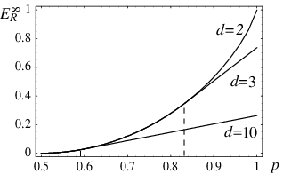
The remarkable behavior of $E_{R}^{\infty}(\sigma(p))$ is shown in Fig. 1 for several values of $d$. The nonlinear behavior for small values of $p$ goes over into a linear dependence on $p$ above the threshold value $p^{\prime}=(d+2)/2d$. An immediate consequence of the result is that there are no inseparable Werner states with zero entanglement cost—a similar conclusion could not be drawn from Rains’ bound as it is not an asymptotic quantity. It is astonishing that, as long as $p\leq p^{\prime}$, $E_{R}^{\infty}$ is invariant under the strongly irreversible operation of twirling, mapping Werner states on ${\mathbb{C}}^{2}\otimes{\mathbb{C}}^{2}$ to Werner states on ${\mathbb{C}}^{d}\otimes{\mathbb{C}}^{d}$ [15].

Interestingly, the dependence of $E_{R}^{\infty}(\sigma(p))$ on $p$ is quite similar to the conjectured behavior of the entanglement of formation for a single copy of an isotropic state [16]: there, one can also distinguish between two regimes, and for larger values of the weight $F$ of the maximally entangled state in the isotropic state the dependence of the entanglement of formation is conjectured to be linearly dependent on $F$.

In this Letter we have concentrated on the important class of Werner states. With similar methods, one can also investigate other classes with high symmetry. It is hoped that this work can significantly contribute to the quest for a better understanding of the asymptotic regime of entanglement.

We would like to thank R.F. Werner and D. Jonathan for fruitful discussions, and E. Rains for drawing to our attention possible connections with [11]. This work was partially supported by EPSRC, The Leverhulme Trust, DFG, the European Union EQUIP project& the ESF QIT program and grants MEC (AP99), IUAP-P4-02 and GOA-Mefisto-666 .

References

- [1] M.B. Plenio and V. Vedral, Cont. Phys. 39, 431 (1998).
- [2] C.H. Bennett et al Phys. Rev. A 53, 2046 (1996); M.A. Nielsen, Phys. Rev. Lett. 83, 436 (1999); G. Vidal, ibid 83, 1046 (1999); D. Jonathan and M.B. Plenio, ibid 83, 1455 (1999); L. Hardy, Phys. Rev. A 60, 1912 (1999); H.-K. Lo and S. Popescu, Lanl e-print quant-ph/9707038.
- [3] C.H. Bennett, D.P. DiVincenzo, J.A. Smolin, and W.K. Wootters, Phys. Rev. A 54, 3824 (1996).
- [4] E.M. Rains, Phys. Rev. A 60, 173 (1999); ibid 60, 179 (1999).
- [5] V. Vedral, M.B. Plenio, M.A. Rippin, and P.L. Knight, Phys. Rev. Lett. 78, 2275 (1997); V. Vedral and M.B. Plenio, Phys. Rev. A 57, 1619 (1998); V. Vedral, M.B. Plenio, K.A. Jacobs, and P.L.Knight, Phys. Rev. A 56, 4452 (1997); M.B. Plenio, S. Virmani, and P. Papadopoulos, J. Phys. A 33, 193 (2000); M.B. Plenio and V. Vedral, J. Phys. A 34, 6997 (2001).
- [6] For all subadditive measures of entanglement one can show that , see H. Barnum, M.A. Nielsen, and B. Schumacher, Phys. Rev. A 57, 4153 (1998).
- [7] P.M. Hayden et al, Lanl e-print quant-ph/0008134.
- [8] If for all for a given state , then clearly holds.
- [9] R.F. Werner, Phys. Rev. A 40, 4277 (1989).
- [10] M., P. and R. Horodecki, Phys. Rev. Lett. 84, 4260 (2000). Despite many results of this paper being withdrawn, the formula for the Werner states’ logarithm of the negativity is correct.
- [11] E. Rains, Lanl e-print quant-ph/0008047.
- [12] K.G.H. Vollbrecht and R.F. Werner, Lanl e-print quant-ph/0010095.
- [13]
A rigorous argument is as follows. Denote the maximum absolute
value of over by . Then
the error
because lies between the bounds . The last term is proportional to the mean absolute deviation from the mean, which is always less than the standard deviation (this follows from the concavity of ). Hence . In the case at hand, is of order : from the definition of , from Eq. (12) the maximal absolute value of equals , and, as can be seen from Eq. (The asymptotic relative entropy of entanglement), the values of and are independent of . Hence, in the limit , the error goes to zero as . - [14] S. Boyd and L. Vandenberghe, Introduction to Convex Optimization, Lecture Notes, Stanford University, 2000/2001.
- [15] The twirling operation in dimensions, , is defined as for states , where the integral is performed with respect to the Haar measure, . Under twirling, Werner states on with weight of the antisymmetric state – regarded as states on – will be mapped on Werner states on with the same weight .
- [16] B.M. Terhal and K.G.H. Vollbrecht, Phys. Rev. Lett. 85, 2625 (2000).