Optimal quantum estimation of the coupling between two bosonic modes

How effectively may we estimate the strength of a simple interaction such as the transmittivity of a beam splitter or the phase-shift imposed in the internal arms of an interferometer ? The Hamiltonian describing the bilinear coupling between two bosonic modes has the form

$$H=\kappa(a^{{\dagger}}b+b^{{\dagger}}a)\>,$$

(1)

where $\kappa$ depends on the specific interaction under consideration. By using the Schwinger representation of the $SU(2)$ Lie algebra, with generators

$$J_{x}=\frac{1}{2}(a^{{\dagger}}b+b^{{\dagger}}a)\>,\quad J_{y}=\frac{1}{2i}(a^{{\dagger}}b-b^{{\dagger}}a)\>,\quad J_{z}=\frac{1}{2}(a^{{\dagger}}a-b^{{\dagger}}b)\>,$$

(2)

we can rewrite the Hamiltonian as $H=2\kappa J_{x}$ and the evolution operator as

$$U_{\psi}=\exp(-{\rm i}J_{x}\psi)\>,$$

(3)

where the global coupling constant $\psi$ is equal to $2\kappa\Delta t$, $\Delta t$ being the effective interaction time. The evolution in Eq. (3) describes, for example, the interaction of two light modes in a beam splitter with transmittivity $\tau=\cos^{2}\psi$ [1], or, apart from a fixed rotation, the evolution of the arm modes in a Mach-Zehnder interferometer, with $\psi$ representing the phase-shift between arms [2, 3]. If the initial preparation of two modes is described by the density matrix $\rho_{0}$ the evolved state in the interaction picture is given by

$$\rho_{\psi}=\exp(-{\rm i}J_{x}\psi)\rho_{0}\exp({\rm i}J_{x}\psi)\>.$$

(4)

In this paper we devote our attention to the estimation of $\psi$ through measurements performed on $\rho_{\psi}$. We denote the generic POVM for such estimation process by ${\rm d}\nu(\phi)$, such that the outcomes of the measurement are distributed according to

$$p(\phi|\psi){\rm d}\phi={\rm Tr}[\rho_{\psi}{\rm d}\nu(\phi)]\>,$$

(5)

where $p(\phi|\psi)$ represents the conditional probability of registering the outcome $\phi$ when the true value of the parameter is $\psi$.

Our objective is to find the best strategy, i.e. the POVM that provides the optimal estimation of the parameter $\psi$ [5]. Since $\psi$ is manifestly a phase-shift, we can use general results from phase estimation theory, which provides the optimal POVM to estimate the phase-shift induced by a phase generator, i.e. a selfadjoint operator with discrete, equally spaced, spectrum. The optimality criterion is given in terms of the minimization of the mean value of a cost function [5] that assesses the quality of the strategy, i.e. it weights the errors in the estimates. Since a phase-shift is a $2\pi$-periodic parameter, the cost function must be a $2\pi$-periodic even function of $(\psi-\phi)$, i.e. it has Fourier expansion with cosines only. The appropriate concavity properties of the cost function are reflected by expansion coefficients which are all negative apart the irrelevant additive constant. A cost function with such Fourier expansion has been firstly considered by Holevo [4], and for such reason it is usually referred to as belonging to Holevo’s class. Notice that the optimal POVM for a given state $\rho_{0}$ is the same for every cost function in this class. A more general quantum estimation approach for different kinds of phase-shift and general quantum system is given in Ref. [6]. There, it is also shown that the kind of problem we are presently dealing with is, in a certain sense, the best situation, since the spectrum of our phase generator is the whole set of integers ${\Zset}$, including negative ones. In this case, there is an optimal orthogonal projective POVM, which can be regarded as the spectral resolution of a self-adjoint phase operator. However, if the estimation is performed with the constraint of bounded or fixed energy, the optimal POVM and the optimal input state $\rho_{0}$ do not correspond to a canonical quantum observable scheme [7]. Moreover, in general the optimal POVM depends on the input state, and the optimal POVM of Ref. [4, 5] holds only for pure states, whereas a generalization to a class of mixed states, the so-called phase-pure states, has been considered in Ref. [6, 8].

The optimal POVM, in the sense described above, provides an unbiased estimation of $\psi$ for preparation $\rho_{0}$ of the two modes, in formula

$$\langle\phi\rangle=\psi\quad{\rm with}\quad\langle\phi\rangle=\int_{0}^{2\pi}\phi\>{\rm Tr}[\rho_{\psi}\>{\rm d}\nu(\phi)]\qquad\forall\rho_{\psi}=U_{\psi}\rho_{0}U^{\dagger}_{\psi}\>.$$

On the other hand, we want also to find the optimal state $\rho_{0}$ for the estimation of $\psi$ according to some cost function, which quantifies the noise of the estimation. The customary root mean square is not a good choice for a cost function, since the function $(\phi-\psi)^{2}$ is not $2\pi$-periodic. A good definition for the precision of the measurement is given by the average of the cost function $C(\phi-\psi)=4\sin^{2}(\frac{\phi-\psi}{2})$, i. e. a ”periodicized variance”, which obviously belongs to the Holevo’s class. If the estimates occur within a small interval around the true value of the parameter $\psi$, one has approximately $C(\phi-\psi)\simeq(\phi-\psi)^{2}$, whence $\delta\psi=\sqrt{C}$ can be assumed as a reasonable measure of the precision of the measurement.

In order to solve our estimation problem, let us consider the following unitary transformation

$${\cal U}=\exp\left\{-\frac{\pi}{4}(a^{{\dagger}}b-b^{{\dagger}}a)\right\}=\exp\left\{-{\rm i}\frac{\pi}{2}J_{y}\right\}\>.$$

(6)

Using Eq. (6) we may rewrite Eq. (5) in the more familiar form of rotation along the z-axis

	$\displaystyle p(\phi|\psi){\rm d}\phi$	$\displaystyle=$	$\displaystyle{\rm Tr}\left[{\cal U}\rho_{\psi}{\cal U}^{{\dagger}}\>{\cal U}{\rm d}\nu(\phi){\cal U}^{{\dagger}}\right]$		(7)
		$\displaystyle=$	$\displaystyle{\rm Tr}\left[\exp(-{\rm i}J_{z}\psi){\cal U}\rho_{0}{\cal U}^{{\dagger}}\exp({\rm i}J_{z}\psi)\>{\cal U}{\rm d}\nu(\phi){\cal U}^{{\dagger}}\right]$
		$\displaystyle=$	$\displaystyle{\rm Tr}\left[\exp(-{\rm i}J_{z}\psi)R_{0}\exp({\rm i}J_{z}\psi)\>{\rm d}\mu(\phi)\right]\>,$

where we used the identity ${\cal U}J_{x}{\cal U}^{{\dagger}}=J_{z}$. Equation (7) shows that the problem of estimating the shift generated by $J_{x}$ on the state $\rho_{0}$ is equivalent to that of estimating the same shift generated by $J_{z}$ on the rotated state $R_{0}={\cal U}\rho_{0}{\cal U}^{{\dagger}}$. In particular, any POVM ${\rm d}\nu(\phi)$ to estimate the $J_{x}$-induced shift can be written as $d\nu(\phi)={\cal U}^{{\dagger}}{\rm d}\mu(\phi){\cal U}$, where ${\rm d}\mu(\phi)$ is a POVM for the $J_{z}$-induced shift estimation.

For pure states $R_{0}=|\psi_{0}\rangle\rangle\langle\langle\psi_{0}|$ (in the following we use double brackets for two-mode vectors) the degeneration of the spectrum of $a^{{\dagger}}a-b^{{\dagger}}b$ can be treated using the technique introduced in [6], and the optimal POVM for cost functions in Holevo’s class [4] is proved to be of the form

$${\rm d}\mu(\phi)=\frac{{\rm d}\phi}{2\pi}\>|E_{\phi}\rangle\rangle\langle\langle E_{\phi}|$$

(8)

with the vectors $|E_{\phi}\rangle\rangle$ given by

$$|E_{\phi}\rangle\rangle=\sum_{d\in{\mathbb{Z}}}{\rm e}^{id\phi}\>|d\rangle\rangle\>.$$

(9)

The vectors $|d\rangle\rangle$ are certain eigenvectors of $D=a^{{\dagger}}a-b^{{\dagger}}b$ built by picking up, in every eigenspace ${\cal H}_{d}$ of the eigenvalue $d$, the normalized vector parallel to the projection of $|\psi_{0}\rangle\rangle$ on ${\cal H}_{d}$. In order to be more specific, let us consider an input state of the form

$$|\psi_{0}\rangle\rangle=\sum_{n=0}^{\infty}\psi_{n}^{(0)}|n,0\rangle\rangle+\sum_{n=0}^{\infty}\sum_{d=1}^{\infty}\left[\psi_{n}^{(d)}|n,d\rangle\rangle+\psi_{n}^{(-d)}|n,-d\rangle\rangle\right]\>,$$

(10)

where $|n,d\rangle\rangle$ is given by

$\displaystyle|n,d\rangle\rangle\equiv\left\{\begin{array}[]{cc}|n+d\rangle_{a}|n\rangle_{b}&{\rm if}\>\>d\geq 0\\ |n\rangle_{a}|n-d\rangle_{b}&{\rm if}\>\>d<0\end{array}\right.\>.$

The projection of $|\psi_{0}\rangle\rangle$ in ${\cal H}_{d}$ is equal to

$$\sum_{n=0}^{\infty}\psi_{n}^{(d)}\>|n,d\rangle\rangle\>,$$

(14)

such that the eigenvector $|d\rangle\rangle$ reads as follows

$$|d\rangle\rangle=\frac{\sum_{n=0}^{\infty}\psi_{n}^{(d)}|n,d\rangle\rangle}{\sqrt{\sum_{n=0}^{\infty}\left|\psi_{n}^{(d)}\right|^{2}}}\>,$$

(15)

and the input state can be rewritten as

$$|\psi_{0}\rangle\rangle=\sum_{d\in{\mathbb{Z}}}\gamma_{d}\>|d\rangle\rangle\qquad\gamma_{d}=\sqrt{\sum_{n=0}^{\infty}\left|\psi_{n}^{(d)}\right|^{2}}\>.$$

Notice that the dependence of the POVM on the state $|\psi_{0}\rangle\rangle$ is contained in the vectors $|E_{\phi}\rangle\rangle$.

By adopting $C(\phi-\psi)$ as a cost function the average cost of the strategy corresponds to the expectation value of the cost operator $C=2-{\rm E}_{+}-{\rm E}_{-}$, where the raising and lowering operators $E_{+}$ and $E_{-}$ are given by

$${\rm E}_{+}=\sum_{d\in{\mathbb{Z}}}|d+1\rangle\rangle\langle\langle d|\qquad{\rm E}_{-}={\rm E}_{+}^{{\dagger}}$$

(with the vectors $|d\rangle\rangle$ defined as above).

The optimization problem is that of minimizing the average cost of the strategy

	$\displaystyle\bar{C}=\int_{0}^{2\pi}\frac{d\psi}{2\pi}\>\int_{0}^{2\pi}\frac{d\phi}{2\pi}\>C(\phi-\psi)\>p(\phi|\psi)={\rm Tr}\left[R_{0}\>C\right]\equiv\langle\langle\psi_{0}|2-{\rm E}_{+}-{\rm E}_{-}|\psi_{0}\rangle\rangle$
	$\displaystyle\;,$		(16)

with the constraint that the solution is a normalized state. The Lagrange function is given by

$${\cal L}=\bar{C}-\lambda\langle\langle\psi_{0}|\psi_{0}\rangle\rangle\;,$$

(17)

with $\lambda$ being the Lagrange multiplier for the normalization constraint. The solution of this problem is a state with infinite mean energy $N=\langle\langle\psi_{0}|a^{{\dagger}}a+b^{{\dagger}}b|\psi_{0}\rangle\rangle$. In order to find physically realizable states, one must impose a constraint on $N$ too, and the Lagrange function becomes

$${\cal L}=\bar{C}-\mu\langle\langle\psi_{0}|a^{{\dagger}}a+b^{{\dagger}}b|\psi_{0}\rangle\rangle-\lambda\langle\langle\psi_{0}|\psi_{0}\rangle\rangle\>,$$

(18)

$\mu$ being the Lagrange multiplier for the mean energy. It is useful, in order to calculate the solution of this equation, to write the generic state $|\psi_{0}\rangle\rangle$ in the following way

$$|\psi_{0}\rangle\rangle=\sum_{d\in{\mathbb{Z}}}\psi_{d}\sum_{n=0}^{\infty}c_{n,d}|n,d\rangle\rangle\>.$$

(19)

The coefficients $c_{n,d}$ determine the normalized projection of $|\psi\rangle\rangle$ into the eigenspace ${\cal H}_{d}$, whereas the $\psi_{d}$’s are the coefficients which combine those projections.

Using Eq. (19), the Lagrange function (18) explicitly shows terms accounting for the normalization of the vectors $\sum_{n=0}^{\infty}c_{n,d}|n,d\rangle\rangle$ in each ${\cal H}_{d}$, with $\nu^{(d)}$ denoting Lagrange multipliers for the normalization of projections, and rewrites as

	$\displaystyle{\cal L}$	$\displaystyle=$	$\displaystyle\sum_{d\in{\mathbb{Z}}}\left\{2|\psi_{d}|^{2}\sum_{n=0}^{\infty}|c_{n,d}|^{2}-\left(\bar{\psi}_{d}\sum_{n=0}^{\infty}|c_{n,d}|^{2}\right)\left(\psi_{d-1}\sum_{m=0}^{\infty}|c_{m,d-1}|^{2}\right)+\right.$		(20)
			$\displaystyle-\left(\bar{\psi}_{d}\sum_{n=0}^{\infty}|c_{n,d}|^{2}\right)\left(\psi_{d+1}\sum_{m=0}^{\infty}|c_{m,d+1}|^{2}\right)+$
			$\displaystyle\left.-\mu|\psi_{d}|^{2}\sum_{n=0}^{\infty}|c_{n,d}|^{2}(2n+|d|)-\lambda|\psi_{d}|^{2}\sum_{n=0}^{\infty}|c_{n,d}|^{2}-\nu^{(d)}\sum_{n=0}^{\infty}|c_{n,d}|^{2}\right\}\>.$

By taking derivatives of the Lagrange function with respect to $c^{*}_{n,d}$ and $\psi^{*}_{d}$ with the constraints

	$\displaystyle\sum_{n=0}^{\infty}|c_{n,d}|^{2}=1\qquad\sum_{d\in{\mathbb{Z}}}|\psi_{d}|^{2}=1$
	$\displaystyle\sum_{d\in{\mathbb{Z}}}\sum_{n=0}^{\infty}|\psi_{d}|^{2}|c_{n,d}|^{2}(2n+|d|)=N\>,$		(21)

and by rephasing the $|d\rangle\rangle$’s we arrive at the system

$\displaystyle\left\{\begin{array}[]{l}(2-\lambda)\psi_{d}-\psi_{d-1}-\psi_{d+1}-\mu\sum_{n=0}^{\infty}(2n+|d|)|c_{n,d}|^{2}\psi_{d}=0\\ \left[(2-\lambda)\psi_{d}^{2}-2(\psi_{d}\psi_{d-1}+\psi_{d+1}\psi_{d})-\mu\psi_{d}^{2}(2n+|d|)-\nu^{(d)}\right]c_{n,d}=0\end{array}\right.$

The second equation in (2) implies that for a fixed $d$ only one coefficient $c_{n,d}$ can be different from zero, say for the value $\bar{n}$, and in this case $|c_{\bar{n},d}|=1$ ¹¹ 1 Indeed, let us suppose $c_{n,d}\neq 0$ for two values $n_{1}=m$ and $n_{2}=p$. Then we must have $(2-\lambda)\psi_{d}^{2}-2(\psi_{d}\psi_{d-1}+\psi_{d+1}\psi_{d})-\mu\psi_{d}^{2}(2p+|d|)-\nu^{(d)}=0$ which implies $2\mu(m-p)\psi_{d}=0$. Since the case $\mu=0$ is not interesting and $\psi_{d}=0$ would imply that the choice of the $c_{n,d}$ is completely arbitrary and irrelevant, the only possibility is $m=p$..

The first equation of (2) can therefore be rewritten as

$$(2-\lambda)\psi_{d}-\psi_{d-1}-\psi_{d+1}-\mu(2n(d)+|d|)\psi_{d}=0,$$

(25)

which allows us to obtain from the second one

$$\nu^{(d)}=-\psi_{d}(\psi_{d+1}+\psi_{d-1})\>.$$

(26)

The solutions of Eq. (26) give local minima for the average cost $\bar{C}$, and one should solve the equation (25) for arbitrary choices of $n(d)$, looking for the optimal one. In the case $n(d)=0$ we have

$\displaystyle\frac{2(\lambda^{\prime}+|d|)}{\frac{2}{\mu^{\prime}}}\psi_{d}=\psi_{d-1}+\psi_{d+1}\>,$

(27)

where $\mu^{\prime}=-\mu$ and $\lambda^{\prime}=\frac{2-\lambda}{\mu^{\prime}}$. Eq. 27 is the recursion equation for Bessel functions, with solution given by

$$\psi_{d}={\cal N}^{-1/2}(\mu^{\prime},\lambda^{\prime})J_{\lambda^{\prime}+|d|}\left(\frac{2}{\mu^{\prime}}\right),$$

(28)

with ${\cal N}(\mu^{\prime},\lambda^{\prime})=\sum_{d\in{\mathbb{Z}}}J_{\lambda^{\prime}+|d|}^{2}\left(\frac{2}{\mu^{\prime}}\right)$ and with the boundary conditions $J^{\prime}_{\lambda^{\prime}}(2/\mu^{\prime})=0$, i.e. $J_{\lambda^{\prime}+1}=J_{\lambda^{\prime}-1}$. Finally, to obtain the optimal state $\rho_{0}$ one has to rotate $R_{0}=|\psi_{0}\rangle\rangle\langle\langle\psi_{0}|$ by the unitary transformation (6).

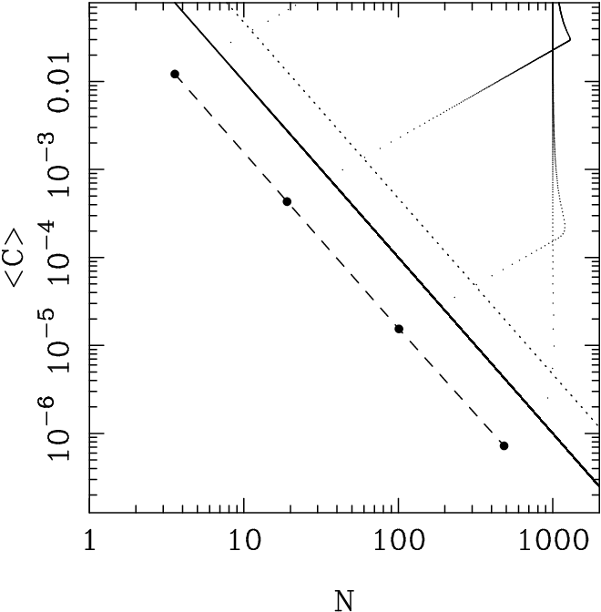
In order to obtain the behaviour of the average cost versus the energy we numerically solved Eq. (25) with $n(d)=0$. This problem can be rewritten as the eigenvalue problem ${\bf A}\psi=\lambda\psi$ for the matrix ${\bf A}$ with elements given by

$$({\bf A})_{m,n}=(2-\mu|m|)\delta_{m,n}-\delta_{m,n+1}-\delta_{m,n-1}\>.$$

(29)

Numerical diagonalization gives the power-law $\bar{C}\simeq\frac{\gamma}{N^{2}}$ in the range $0\lesssim N\lesssim 1000$ with $\gamma\simeq 0.1$. This behaviour is plotted in Fig. 1, where also other solutions of equation (25) corresponding to local minima of the average cost are shown. Since the phase distribution of the optimal state is singly peaked we may also write $\delta\psi\simeq\sqrt{\bar{C}}\simeq\gamma^{1/2}/N$, which means that the optimal states derived here are at the so-called Heisenberg limit of phase variance.

In conclusion, we dealt with the problem of estimating the coupling constant of a bilinear interaction. In our approach the coupling constant, which appears in the exponent of the time evolution operator, has been treated as a phase parameter. The optimal POVM has been derived according to the theory of quantum phase estimation [4, 5, 6, 8]. As noticed in Ref. [2] this resorts to an SU(2) estimation problem with the Schwinger two-mode boson realization. However, the representation is not irreducible, and a more complicated problem is faced. In this sense our results generalize those of Ref. [2], where the estimation of $SU(2)$ phase-shifts has been analyzed in irreducible subspaces: indeed we found an improved scaling of phase variance versus the total energy. The degeneracy of the spectrum of the the Hamiltonian, can be treated using the technique of Ref. [6], and, in this way, the problem is reduced to a nondegenerate one with spectrum ${\mathbb{Z}}$ for the phase-shift operator.

It is important to remark that the optimal POVM depends on the preparation state. This is true for every kind of phase estimation problem, but in the presence of degeneracy the dependence is crucial. In fact, one has to define the optimal POVM as a block diagonal operator, where the invariant subspaces are spanned by projections of the input state into the eigenspaces of the generator. From a practical point of view this means that optimal estimation of the phase-shift imposed to a state, needs a measuring device which is adapted to the shifted state. We then optimized the input state by minimizing the average cost for fixed input energy and found a power law $\delta\psi\simeq\gamma/N$ in a range $0\lesssim N\lesssim 1000$.

Notice that the law $N^{-1}$ is the same as in the optimal phase estimation with only one mode [9], however with a much smaller constant $\gamma$ ($\gamma\simeq 0.1$ instead of $\gamma\simeq 1.36$). We think that this phenomenon of improvement of phase sensitivity by increasing the number of modes is the same considered in Ref. [10], where an exponential improvement versus the number of modes has been estimated when increasing the number of modes and the the number of photons per mode, jointly in the same proportion.

This work has been cosponsored by MURST under the project ”Quantum Information Transmission and Processing”. The authors thank Dipartimento di Fisica ”Alessandro Volta” for partial support.

References

- [1] L. Mandel, E. Wolf Optical Coherence and Quantum Optics (Cambridge University Press, 1995).
- [2] B. C. Sanders, G. J. Milburn, Phys. Rev. Lett. 75, 2944 (1995).
- [3] M. G. A. Paris, Phys. Rev. A 59, 1615 (1999).
- [4] A. S. Holevo, Probabilistic and Statistical Aspects of Quantum Theory (North-Holland Publishing, Amsterdam, 1982).
- [5] C.W.Helstrom, Found. Phys. 4, 453 (1974); Int. J. Theor. Phys. 11, 357 (1974); Quantum Detection and Estimation Theory (Academic Press, New York, 1976)
- [6] G. M. D’Ariano, C. Macchiavello, and M. F. Sacchi, Phys. Lett. A, 248 103 (1998).
- [7] M. G. A. Paris, Nuovo Cimento B 111, 1151 (1996).
- [8] G. M. D’Ariano, C. Macchiavello, P. Perinotti, and M. F. Sacchi, Phys. Lett. A, 268 241 (2000).
- [9] G. M. D’Ariano e M. G. A. Paris, Phys. Rev. A 49, 3022, (1994).
- [10] H. P. Yuen in Squeezed States and Uncertainty Relations, D. Han et al Eds. NASA CP 3135, p 13 (1992).