Quantum coherence and control in one- and two-photon optical systems
Abstract
We investigate coherence in one- and two-photon optical systems, both theoretically and experimentally. In the first case, we develop the density operator representing a single photon state subjected to a non-dissipative coupling between observed (polarization) and unobserved (frequency) degrees of freedom. We show that an implementation of “bang-bang” quantum control protects photon polarization information from certain types of decoherence. In the second case, we investigate the existence of a “decoherence-free” subspace of the Hilbert space of two-photon polarization states under the action of a similar coupling. The density operator representation is developed analytically and solutions are obtained numerically.
[Note: This manuscript is taken from the author’s undergraduate thesis (A.B. Dartmouth College, June 2000, advised by Dr. Walter E. Lawrence), an experimental and theoretical investigation under the supervision of Dr. Paul G. Kwiat.11 1 Physics Division, P-23, Los Alamos National Laboratory, Los Alamos, NM 87545, USA. Email: kwiat@lanl.gov.]
I Introduction
Decoherence in two-state quantum systems is a significant obstacle to the realization of proposed quantum information technologies. Coupling between quantum bit (“qubit”) states and unobserved environmental degrees of freedom leads to decoherence effects which limit the practical implementation of proposed quantum algorithms unruh. Photon modes, including polarization and spatial modes, provide an easily accessible system in which simple quantum circuits can be investigated unitary; opticalqubits; grover. Here, we examine the process of decoherence by subjecting single photons to a controllable birefringent “environment” and observing the evolution of the polarization state.
In section II, we investigate the evolution of a single photon state under the action of a unitary coupling between polarization and frequency modes. Such non-dissipative “phase errors” give rise to decoherence effects, whereby the photon evolves from a definite polarization state to an unpolarized state. We then introduce and examine an optical implementation of so-called “bang-bang” quantum control of decoherence by rapidly exchanging the eigenstates of the coupling operation bang-bang. The term “quantum control” is justified since such an operation will be shown to preserve a coherent polarization state in some special cases, and to reduce decoherence in more general cases.
In section III we will introduce a particular two-photon polarization-entangled state that, due to its symmetry properties, is immune to collective decoherence of the type mentioned above. That is, this state is a decoherence-free subspace (DFS) of the Hilbert space of photon polarization zanardi; lidar. Photon pairs entangled in both polarization and frequency degrees of freedom, such as hyper-entangled photons produced in down-conversion sources (see source; ultrabright), further complicate this particular decoherence mechanism . In particular, energy conservation imposes frequency correlations which affect the coherence properties of these two-photon states. In the experimental case, it will be shown that this frequency correlation can be effectively suppressed and the DFS recovered by a simple and physically intuitive modification of the apparatus.
II Coherence and “bang-bang” control: The one-photon case
II.1 Review of single-photon decoherence
In this section, we will show that non-dissipative (unitary) coupling between photon frequency and polarization in a birefringent ‘‘environment’’ followed by a trace over frequency leads to decoherence.22 2 This effect has a well-known counterpart in classical optics whereby quasi-monochromatic light composed of uncorrelated frequency components loses the ability to interfere with itself when polarization modes are separated beyond the coherence length of the incident light, as in an unbalanced Michelson interferometer (see born_and_wolf, 7.5.8). These results are relevant to the study of decoherence in quantum systems which arises when coupling to environmental states, followed by a trace over those degrees of freedom, leads to a loss of phase information between qubit basis states. In the following argument, the term “environmental” will be used to describe the coupling of information-carrying states (photon polarization modes) to degrees of freedom which are not utilized for information representation (photon frequency modes). It will be shown that even non-dissipative coupling between these modes leads to a loss of information in the qubit states.
A single photon characterized by its frequency spectrum and polarization can be represented by the state ket
| (1) |
where are orthonormal polarization basis states with complex amplitudes , and is the complex amplitude corresponding to the frequency , normalized so that
| (2) |
For simplicity, we assume that the frequency spectrum is independent of polarization, so that we need not index by polarization mode. In physical terms, this means that polarization and frequency are not entangled.
Since represents a pure state, the density operator can be written as (see sakurai, 3.4), so that we have the initial state
| (3) | |||||
The subscript indicates that includes frequency degrees of freedom. The usual density matrix representing the polarization state of the photon is given by .
We will now seek the dependence of the density operator on some spatially extended “environment,” by introducing the operator which we require to be both linear and unitary. Furthermore, we demand that have eigenkets with (frequency-dependent) eigenvalues where, as before, indexes the polarization mode. Since exhibits frequency- and polarization-dependent eigenvalues, it introduces a coupling between qubit states (polarization modes) and non-qubit states (frequency modes). As shown in Appendix A.1, introduces pure“phase errors” on polarization modes , so that
| (4) |
where the phase factor is a real-valued function of and .
Now we can calculate the spatial dependence of the density operator under the influence of and following a frequency-insensitive measurement, effected by a partial trace over frequency degrees of freedom:
| (5a) | |||||
| (5b) | |||||
Since this process realizes the entangling of qubit states with environmental states (frequency modes which are not involved in information representation or manipulation), we expect to observe decoherence effects in the off-diagonal elements of the qubit state (polarization) density matrix zanardi. In order to investigate the coherence properties of a photon under the action of such an operator, we observe that in a completely mixed (or “decohered”) state, the density matrix is simply a multiple of the identity matrix. The diagonal elements of are indexed by . For these values of and , the argument of the exponential in Eq. 5b vanishes and by the normalization condition (Eq. 2), we have . In other words, the diagonal elements of are unaffected by .
The off-diagonal elements of the density matrix are indexed by the values and . To compute these explicitly, we must define the functions . In the case of a single photon in a birefringent, linearly dispersive crystal of thickness (e.g., a quartz crystal),
| (6) |
where is the index of refraction corresponding to polarization .33 3 Here, we neglect dispersion, the variation of with . By assuming to be an eigenstate of (Eq. 4), we require the optic axis of the birefringent element to be aligned with one of the polarizations . In the case where the represent circular (elliptical) polarizations, this means that the environment is optically active as opposed to (as well as) birefringent. Making the substitution and writing , the off-diagonal elements of the density matrix are given by
| (7a) | |||||
| (7b) | |||||
where is the Fourier transform of (up to a constant, depending on convention).
Evidently, implies that , so that Eqs. 7a and 7b preserve the required hermiticity of . In terms of and , the density matrix at some later position becomes a simple modification of the density matrix at :
| (8) |
Eq. 8 allows us to calculate the density matrix representing the polarization of an optical qubit subjected to a non-dissipative frequency-polarization coupling, given the initial state density matrix, , (written in the basis of eigenmodes of the coupling) and the functional form of the frequency-amplitude function .44 4 Actually, we need only know the complex square of the frequency-amplitude function, . In general, is peaked at some central value with a finite width . Under these conditions, the Fourier transform (and the off-diagonal elements of ) will fall significantly on the time scale . In other words, there is no coherent phase relationship between polarization basis states and after the photon has traveled a distance through the environment .
To summarize, we have developed a prescription for calculating the polarization state density matrix representing a photon in a birefringent environment. From this expression, we see that a photon with definite polarization phase information before entering such an environment will, in general, lose phase information between polarization basis states after traveling a suitably long distance. The physical mechanism which destroys such phase information is the entanglement between polarization modes and frequency modes, which is an instance of the entanglement between qubit states and environmental degrees of freedom which are not useful for information manipulation. Because we trace over frequency (environmental) degrees of freedom in this case, the phase coherence between the qubit basis states is destroyed.
II.2 “Bang-bang” quantum control of decoherence
In the previous section, we showed that a qubit consisting of photon polarization modes may lose its capacity for information representation under the action of a unitary operator, , which entangles frequency and polarization. In other words, decoherence occurs even for non-dissipative “phase errors” in which the qubit basis states are eigenstates of the environmental coupling, and there is no chance for a bit flip error unruh.55 5 Note however, that phase errors in the basis may appear as bit-flip errors in another basis, e.g. .
In bang-bang, the authors describe this result in the general case of qubit states coupled to environmental degrees of freedom and introduce a scheme for reducing such decoherence effects via rapid, periodic exchanging of the eigenstates of the environmental coupling. In our case, this corresponds to an interchange of the polarization basis states and , which can be accomplished by an appropriate reflection or rotation operation. These exchanges are rapid in the sense that the period of flipping must be short compared to the decoherence time and the time scales of any other relevant decoherence mechanisms (e.g. scattering, dissipation). So called “bang-bang” control reduces the degree of decoherence by averaging out the time-dependent coupling between qubit states and environmental states.
In this section, the previous results are expanded to include an implementation of “bang-bang” quantum control by periodic exchanging of the environmental eigenstates . The mathematical formulation is considerably simplified if we move to the discrete regime in which the ‘‘environment’’ acts in a stepwise fashion, and the exchange of eigenstates also occurs in discrete steps.66 6 Developing the general continuous case in analogy with Sect. II.1 by including a rotation operator acting simultaneously with is considerably complicated, since this rotation operator will not, in general, commute with for different values. To this end, we define to be a reflection (or rotation) operator which exchanges the eigenstates of the frequency-polarization coupling:
| (9a) | |||||
| (9b) | |||||
Here, the plus (minus) sign refers to a reflection (rotation). The choice of sign will not affect the results of a measurement in the experimental case, and for concreteness, we take the sign to be positive.
We define , a “step-wise” operator analogous to in Sect. II.1 and also define to be the thickness of the birefringent element (in our experiments, usually a quartz crystal); as before, is the refractive index corresponding to polarization state , and . This gives a relative phase shift of , so that we have77 7 Here, we omit the phase shift of , which is common to Eqs. 10a and 10b. Such a global phase shift is never observable and cannot affect the coherence properties of the polarization states.
| (10a) | |||||
| (10b) | |||||
Eqs. 9a-9b and 10a-10b have the important consequence that
| (11a) | |||||
| (11b) | |||||
where it is understood that such operator identities are only meaningful when the operators are applied to kets or bras (see Appendix A.2.1 for a proof of these identities).
In this discrete regime, we consider “rapid” exchanging of eigenstates to correspond to the alternating action of the operators and . Regarding and as optical elements (for example, a quartz crystal and a half-wave plate), we consider a cavity scheme in which a single photon passes through this two-element unit times.
Symbolically, after passes through the system, we have (compare Eq. 5a),
| (12) |
Application of identities 11a and 11b leads to a simplification, depending on whether is odd () or even ().
| (13a) | |||||
| (13b) | |||||
Note that is related to the continuous case of Sect. II.1 by
| (14) |
These relations lead to a simple analog of Eq. 5b (where we use , given by Eq. 3, as the input state in both cases):
| (15a) | |||||
Finally, writing out in matrix form, substituting for the Fourier transform of , and denoting by the characteristic time parameter, we have
| (16a) | |||||
The subscript (for “Quantum Control”) indicates the case in which is included. Note that is dependent only on the parity of , so that under the influence of the quantum control procedure, any number of cycles through this particular birefringent environment causes at most a decoherence equal to that of the first pass. In fact, Eq. 16a shows that an even number of cycles causes no decoherence whatsoever.
By making the identification (the distance traveled through the crystal after N passes) in Eq. 8, we can directly compare the results of Sect. II.1 with those of Sect. II.2:
| (17) |
Letting be the coherence time such that is significantly reduced for , then represents a partially mixed state for .88 8 Here, “mixed” refers to the fact that the off-diagonal elements of are small so that . If the initial state, , has diagonal elements of , then represents a completely random ensemble for . On the other hand, never loses all phase information in the off-diagonal elements since recovers the initial state for all . In this sense, acts as a quantum control element, suppressing decoherence and maintaining state purity indefinitely.
We may ask what happens if the strength of the environmental coupling varies with , so that varies on a time scale comparable to the period of the exchange operator, . For simplicity, we model this “slow-flipping” case by introducing two distinct operators which differ only in their eigenvalues (not their eigenstates). In more concrete terms, we consider two coupling operators, and , characterized by phase errors and so that, for :
| (18a) | |||||
| (18b) | |||||
The exchange operator acts in alternation between each of these two operators, so that the strength of the coupling changes faster than the eigenstates of the coupling are exchanged. After N passes through the system, we have
| (19a) | |||||
Intuitively, we expect to see a partial reduction in the degree of decoherence when the quantum control procedure is implemented by introducing the exchange operator.
To see these results quantitatively, we make the following substitution which reduces this problem (mathematically) to the previously solved one (see Appendix A.2.2 for a derivation of these relations):
| (20a) | |||||
| (20b) | |||||
so that,
| (21a) | |||||
| (21b) | |||||
| (22a) | |||||
| (22b) | |||||
With these relations, each operator is mathematically analogous to the operator defined by Eq. 4, with redefined as appropriate given relations 21a-22b and the details of the particular environment. In the case of birefringent crystals, the elements corresponding to and differ only in their thickness (not in their orientation with respect to the polarization basis states ). Defining to be the thickness of a crystal represented by , we have
| (23) |
We see that before introducing the exchange operator, the birefringent environment acts effectively as a single birefringent crystal of thickness (Eq. 21b). After implementing “bang-bang” control by introducing the exchange operator , the environment looks effectively like a single crystal of thickness (Eq. 22b). In the absence of quantum control, the photon is subjected to the sum of the individual phase errors; in the presence of a quantum control element, the photon is subjected to the difference of the individual phase errors. In this case, where the strength of the environmental coupling changes on roughly the same time scale as the exchanging of eigenstates, the quantum control procedure reduces but does not eliminate decoherence effects.
II.3 Experimental Demonstration of “Bang-Bang” Control
It will be convenient in our experimental analysis to measure the visibility, traditionally defined as
| (24) |
where () denotes the maximum (minimum) number of photons passing through orthogonal settings of a polarizer. Denoting these polarization analyzer settings by and , we define visibility at the single quantum level by calculating probabilities from the density operator, 99 9 The notation , is intended to suggest that these polarization modes may, in general, represent any elliptical orthonormal basis states.:
| (25) |
Note that we no longer include the denominator corresponding to the total number of photons in Eq. 24, since the denominator here is the trace of in the basis, which is unity. quantifies the similarity between the state represented by and the state in the following sense: if represents an unpolarized state, it is a multiple of the identity matrix, and ; at the opposite extreme, if the photon is in a pure state with polarization , , and . If we choose to measure with respect to the state , we find that (See Appendix A.3 for a proof)
| (26) |
where we have dropped the subscript for this choice of measurement, and indicates the real part. In this form, it is clear that visibility depends on the off-diagonal elements of , and so corresponds with our previous notion of coherence. If we write in the basis, measuring the visibility with respect to and gives us information about the off-diagonal elements of .
To see the results of the previous sections experimentally, we seek a systematic and controllable implementation of the operators and in the cavity scheme of Sect. II.2. For the first case, in which there is a single operation which produces a phase error, we use a Michelson polarization interferometer as a tunable decoherence mechanism in the basis. A polarizing beam-splitter (PBS) separates the path of - and -polarized light. The unbalanced arms of the interferometer produce a controllable, -dependent phase shift between and (see Fig. 1).

A photon in either path is reflected back to the PBS and retraces its path to the input. The difference in path lengths between arms of the interferometer will be denoted by . The unbalanced interferometer is the optical realization of the operator of Sect. II.1 and of Sect. II.2.
An reflector at the input recycles the light so that a photon passes through the unbalanced arms of the interferometer more than once, in general.1010 10 We use to denote the probability of reflection at a surface. A partially reflective out-coupling mirror directs a photon out of the interferometer with a probability of at each pass.1111 11 For normal incidence, at each air-glass interface. Here, one surface of the out-coupling mirror is broad-band anti-reflection (BBAR) coated so that we have effectively only a single air-glass interface.
We send in light from a greatly attenuated diode laser at nm, pulsed at kHz. In our experiment, we observe photons passing through the interferometer times. The total distance traveled by a photon passing through our interferometer times is m, so that any photon spends at most s in the system. EG&G SPCM-AQ silicon avalanche photodiodes (dark count , efficiency ) are used as photon counters. Using electronic timing techniques, we record photon counts only in a coincidence window of 50 ns between the pulse generator and detection event. These timing techniques, together with spectral filters at the detectors, reduce background coincidence counts to s-1. We graphically display photon counts vs. arrival time so that photons leaving the system after N cycles are recorded in the Nth peak. In a typical experiment, our photon counters register no more than coincidence counts per second, and we conclude that photons per second leave the system ( per pulse).1212 12 The probability that there are two photons in the system simultaneously is given by the Poisson distribution, . These photon numbers are comparable to those used in current demonstrations of free-space quantum cryptographic key distributions crypto. At the output, we count for a few seconds (less than a minute in most cases). Although we cannot determine the unknown polarization state of a single photon, we can accurately find the statistical distribution of the ensemble over the observation time, from which useful information about the density matrix can be inferred.
By placing a waveplate with optic axis at at the recycling reflector, we realize an optical “flipping” operator. The -reflector- combination takes to and vice versa. This is the optical realization of the exchange operator, in Sect. II.2.
By recording photon counts in coincidence with the diode pulse generator and using a polarizer at the detector, we can measure the visibility at . The frequency spectrum of laser light is restricted using an interference filter with bandwidth nm and central wavelength nm.1313 13 Since the diode laser is weakly driven just above its lasing threshold, the intrinsic frequency spectrum of the photons is wide enough that these filters determine the overall frequency distribution. For our calculations, we use a Gaussian amplitude function with frequency spread corresponding to nm, central frequency corresponding to nm, and normalization factor :1414 14 In practice, we find that the frequency spectrum is not as smooth as a Gaussian. From the visibility curves, we infer that the frequency spectrum has a substantial monochromatic (compared to ) component at .
| (27) |
The corresponding coherence length of the photons is given by m, so we expect substantial decoherence for a path difference of m at cycle .
| (a) |

|
|---|---|
| (b) |

|
| (c) |

|
With this setup, we can measure vs. N as in Sect. II.2. Experimental and theoretical results are plotted in Fig. 2 for the case where the arms are unbalanced by m. The experimental results show clearly that the introduction of the quantum control element results in a significant reduction of decoherence in good agreement with the theory. However, practical difficulties with the interferometer limit the quantitative agreement between experimental and theoretical values of , especially at large N. We see in Fig. 2(a) that the relative path difference is not 0 after passes through the interferometer due to imperfect balancing. By determining the coherence length from the data in Fig. 2, we infer that the actual path length difference in the interferometer was m (about one wavelength of incident light) displaced from the nominal -values. This discrepancy then determines the bounding value of for all other plots. Theoretically, of course, this value is exactly unity.
In order to model the “slow-flipping” case, we introduce an additional operator, , which will induce a second phase shift, also in the basis. To accomplish this task, we include a birefringent quartz crystal whose optic axis is aligned with the axes of the PBS of the original setup. We denote the optical path difference in this crystal by .1515 15 Instead of a single quartz crystal, we use a 1.046 mm crystal at and a 0.850 mm crystal perpendicular to the first. The combination of these two crystals gives an effective path length such that nearly complete decoherence occurs over 10 cycles. We now use a -waveplate as the quantum control element which exchanges the eigenstates, and , at each pass both to the left and to the right (see Fig. 3). For the theoretical values, we used the same prescription as above, but with effective operators defined by Eqs. 21a-22b. Experimental and theoretical results are displayed in Fig. 4.

| (a) |

|
|---|---|
| (b) |

|
| (c) |

|
In Fig. 5, we have inferred the effective rate of decoherence (a reciprocal length, in this case) in the system by fitting curves to each of Fig. 4 and (reciprocally) plotted these versus the rate of decoherence for a single pass predicted by Eqs. 21b and 22b. We expect to see an effective decoherence rate given by the sum of , the decoherence rate due to the quartz crystal, and , , the decoherence rate due to the interferometer, when the quantum control procedure is not implemented; furthermore, we expect to see a decoherence rate determined by the difference of and when the quantum control procedure is implemented. Here, the decoherence “rate” of an optical element is directly proportional to the reciprocal of the optical path difference between e- and o-polarizations. The linearity of this plot indicates that the quantum control element acts as predicted in Sect. II.2.

We are limited in the type of decoherence we can observe by measuring . For example, a photon in the pure state has a visibility of with respect to the basis. We would like a more general method of quantifying decoherence effects. To this end, we can extend the various methods of polarization analysis in classical optics to our more fundamental quantum mechanical setting. With this idea in mind, we define the degree of polarization , and the Stokes parameters in terms of as1616 16 These are a generalization of the Stokes parameters of classical optics to the quantum mechanical case. In classical optics, these data can be used to reconstruct the coherency matrix, , which completely characterizes the polarization state of the light (See born_and_wolf, ).
| (28) |
and
| (29a) | |||||
| (29b) | |||||
| (29c) | |||||
As usual, and denote horizontal and vertical polarization, denotes polarization, and denotes right-circular polarization.
Note that photon counting in the appropriate polarization basis allows experimental determination of the Stokes parameters, . By photon counting and using the relations 29a-29c, the density matrix of an arbitrary polarization state can be reconstructed from these data.1717 17 An extension of this technique of quantum tomography has been demonstrated by reconstruction of two-photon density matrices in non-max. This technique will be useful in the two-photon state discussions of Sect. III. In contrast to measurements of with respect to some particular orthonormal basis , this tomographic technique allows complete determination of the polarization state. In fact, the visibility with respect to any basis can be found from the density matrix if the transformation from to is known.
In the previous cases, we used an appropriately oriented waveplate as a realization of the exchange operator, . However, the choice of orientation in both cases required prior knowledge of the eigenstates of the coupling between frequency and polarization. Note, however, that if we know only that the eigenstates of the coupling are orthogonal, linear polarization states, then a rotation by (as opposed to reflection about a specific axis) meets the requirements of an exchange operator (Eqs. 9a-9b) in all cases. We expect that an optically active quartz rotator acts as a quantum control element, independent of the orientation of the quartz crystal that causes decoherence (since the eigenstates of our birefringent quartz crystal are orthogonal and linear, i.e., along the optic axes of the crystal).1818 18 If the eigenstates of the environmental coupling are left- and right-circular polarizations, a waveplate at any orientation acts as the exchange operator .

To investigate decoherence in an “adjustable” linear basis, we use a cavity with a photon passing through mm and mm birefringent quartz crystals at each cycle. Since this thickness of quartz results in substantially faster decoherence than the unbalanced interferometer of the previous cases, we use a narrow bandwidth filter of nm to increase the coherence length of the photons. The exchange element, a quartz rotator, is placed between the birefringent crystals (see Fig. 6). At the output, we measure the Stokes parameters by photon counting in the appropriate bases and calculate to quantify the degree of coherence. By orienting both birefringent crystals so that the optic axis makes an angle of with the horizontal, and sending linearly polarized light at into the system (for maximum decoherence), we see that the rotator does indeed act as a quantum control element (Fig. 7). Note however, that we need not rotate the optically active element by a corresponding , because its functionality is independent of such a rotation. Put differently, the rotator acts as a quantum control operator for (slow) decoherence in all linear bases.
For the theoretical curves in Fig. 7, we need not modify the previous calculations except to take the lower (negative) sign in the definition of , Eq. 9b and include the narrower frequency spectrum. The invariance of physical systems under rotation allows us to rotate the entire experimental apparatus (the input polarization and quartz crystals) by without adjusting the calculations.

As a further demonstration of “bang-bang” quantum control of decoherence, we seek a scheme in which the strength and the eigenstates of the polarization-frequency coupling change between exchange operations. To reproduce these conditions, we simply place the quartz crystals of Fig. 6 at slightly different angles so that the eigenstates of the coupling are not constant at each pass. The first (1.0 mm) crystal is oriented at to the horizontal while the second (0.8 mm) crystal is placed at degrees. To solve for starting from the density operator representation, we rewrite the first crystal operator as a matrix in the basis using the appropriate rotation matrices. The resulting output density matrices are calculated numerically and is extracted. The theoretical and experimental results are displayed in Fig. 8.


As a final demonstration of bang-bang control, we assert that the same technique of exchanging orthogonal polarization states will also compensate for decoherence via dissipative (i.e., non-unitary) errors. Experimentally, we accomplish this task by inserting a neutral-density (-independent) filter into the transmission () arm of the balanced Michelson interferometer of Fig. 1. This filter results in loss (after two passes) per cycle. Denoting this operator as , letting , and using the input state , we have, after cycles,
| (30) |
In the case when the quantum control procedure is implemented, and alternate so that the state evolves in the following steps
| (31) | |||||
so that
| (32) |
In this way, we prove the operator identity so that, after an even number of cycles, the system evolves back to its original state but with a reduced probability of detection. Experimental and theoretical results for this case are displayed in Fig. 9.
In summary, we have shown that coupling information-carrying (polarization) degrees of freedom to unobserved (frequency) degrees of freedom results in a loss of polarization phase information. We have shown in this section that an optical realization of ‘‘bang-bang’’ control of decoherence does indeed preserve photon polarization in the presence of such an ‘‘environment.’’ Our implementation of bang-bang control requires some knowledge of the eigenstates of the polarization-frequency coupling. We have demonstrated such control when the eigenstates of the coupling are linear and orthogonal.1919 19 In fact, in the Poincaré Sphere representation of polarization (See born_and_wolf ), it is sufficient to know only the plane in which the eigenstates of the coupling lie: a rotation about the normal to that plane satisfies the conditions of an exchange operator . The technique fails, however, for a decoherence mechanism whose eigenstates coincide with those of (i.e., which are parallel to this normal direction). In addition to preserving polarization phase information in the presence of a frequency-polarization coupling, we have shown that such bang-bang control similarly reduces decoherence when the strength and/or the eigenstates of the coupling vary between exchanges.
III Decoherence-free subspaces of two photons
III.1 Polarization-frequency coupling in correlated photon pairs
It has been shown that the antisymmetric 2-qubit state given by (in our optical notation) is immune to collective decoherence, i.e. decoherence arising from an operation that is invariant under qubit permutations zanardi. That is, due to its symmetry properties, is a decoherence-free subspace (DFS) of 2 qubits. Therefore, it is reasonable that we expect the two-photon polarization state to be immune to decoherence of the type discussed in Sect. II, which arises from coupling to frequency degrees of freedom that are unused for information representation.
In this section, in order to investigate the possibility of a DFS, we will consider polarization phase information in a two-photon system. In non-linear optical materials, spontaneous parametric down-conversion events can be used to produce spatially separated, polarization-entangled photon pairs with high fringe visibility source; ultrabright. Here, we extend the results of Sect. II by presenting a method for calculating the density matrix representing the polarization of such a two-photon state in the presence of a birefringent environment. Experimentally, we use the source detailed in ultrabright which produces correlated photon pairs in the two paths labeled L and R (See Fig. 10, p. 10).
In order to keep track of frequency, spatial mode (L or R), and polarization, we define a shorthand notation for indexing the 44 two-photon density matrix . The element is defined to be where the subscripts L and R refer to the left and right photon paths respectively and and refer to the polarization basis states. As a concrete example, in the basis, the state is written as and is written as . In this way, each of the 16 entries of is indexed by four numbers, (), where .
In order to satisfy energy conservation, the frequencies of photon pairs produced in a down-conversion event must sum to the frequency of the pump beam, and their resultant energies become entangled (see mandel_and_wolf ). Denoting the pump frequency by and the frequency of daughter photon by (), we therefore require
| (33a) | |||||
| (33b) | |||||
so that we have in all cases.2020 20 We have used the notation of franson where such frequency entanglement is shown to cause nonlocal cancellation of dispersion to second order in optical systems. This frequency “anti-correlation” will be important in an experimental demonstration of a DFS.
Taking to be the (in general, complex) amplitude of the state and denoting the frequency spectrum by , we write the initial (pure) state at as2121 21 We impose the normalization condition so that initially and .
For completeness, and to make this indexing scheme explicit, we write the reduced density matrix representing the pure polarization state :
| (35) |
Note that there are six independent parameters corresponding to the four complex amplitudes of the states constrained by the normalization condition and the freedom to choose the global (overall) phase.2222 22 For a partially mixed state, there are 15 independent parameters corresponding to 4 real diagonal elements reduced to 3 by the normalization constraint, and 12 complex amplitudes in the upper right entries.
Introducing the shorthand notation and , the density operator for the initial state, including frequency modes, can be written as
| (36) | |||||
where we must be careful to treat and as functions of the variables of integration and .
In order to represent a birefringent crystal in each path, we define the operator
| (37) |
which depends on the distance, (), traveled through such a crystal in the L (R) photon path. It should be noted that the in Eq. 36 represents a tensor product between the Hilbert spaces of photon polarization and photon frequency, whereas the in Eq. 37 represents the tensor product of photon spatial modes L and R. In analogy with Sect. II.1, associates a frequency-dependent phase, , to each polarization state in the path labeled L:
| (38) |
A similar relation holds for the path labeled R. The functions characterize the phase shift induced in either path (L or R). In this way, we require that the coupling between frequency and polarization share the same dependence on the parameters and in either photon path. This requirement is reasonable since we wish to explore the robustness of the antisymmetric state against collective decoherence.
Making a frequency-insensitive measurement of polarization after the photon in path L (R) has traveled a distance (), we have
| (39) |
which gives
| (40) |
Eq. 40 gives a prescription for calculating the density matrix representing polarization degrees of freedom in the presence of non-dissipative “phase errors.” As in Sect. II.2, we expect to observe decoherence effects in the off-diagonal elements of . Note that for the diagonal elements of , indexed by (see Eq. 35), the argument of the exponential is identically zero so that the diagonal elements do not change. Of course, this result holds only for the case of a unitary frequency-polarization coupling in this particular orientation (i.e., with eigenstates and ).
Let us now choose the functions to be identical to those of Eq. 6. In other words, we choose to realize a unitary polarization-frequency coupling by placing a birefringent crystal across both photon paths with e- and o-axes aligned with and .2323 23 We can realize this situation experimentally either by placing the same crystal across both paths, or equivalently by placing “identical” crystals in each path and at the same orientation. For future convenience, we choose the second option. Letting denote the thickness of the crystal, the phase difference between these functions evaluated at is given by
| (41) |
In Appendix A.4, the density matrix representation is written for the evolution of the Bell states and . From these, we see that the states become “incoherent” in the presence of such a frequency-polarization coupling. Here, we do not make a quantitative measure of coherence (or mixture) but simply observe that the off-diagonal elements of the density matrix approach zero for larger than the coherence length of the down-converted photons, given by where is the width of the frequency spectrum . Therefore, these states lose phase coherence information in the presence of polarization-frequency coupling of this type: identical birefringent crystals in the same orientation in both photon paths.
On the other hand, the states do not undergo decoherence for this particular coupling: they retain a definite phase relationship in the off-diagonal matrix elements. We see from the density matrix representation that the state at the input looks like at the analyzer.2424 24 The phase factor arises from the pump frequency which we have assumed to be effectively monochromatic so that only a definite phase shift, and not decoherence, occurs. Including a frequency spectrum of finite width for the pump would result in additional decoherence effects on a different length scale, the coherence length of the pump beam. For this particular arrangement, a birefringent crystal with axes along and , the states do not decohere: there is no decline in magnitude of the off-diagonal elements of the density matrix.
Note, however, that neither of the states can be considered a decoherence-free subspace (DFS). In general, with respect to another (possibly elliptical) basis ,
| (42) |
In particular, using the basis of left- and right-circular polarization, it can be shown that . So, just as the state loses phase information in a birefringent crystal whose eigenmodes (for photons in either path) are and , the state loses phase information in a crystal whose eigenmodes are and . On these grounds, the only candidate for a DFS is the singlet state , since, in analogy with the spin- singlet state , this state is rotationally invariant and looks the same when written in any basis (see sakurai, ). However, we have already shown that the state loses phase information in this system.
III.2 Recovering a decoherence-free subspace
The apparent contradiction between the prediction of a DFS and the contrary result in the previous section arises as a result of the frequency entanglement (anti-correlation) in down-converted photon pairs. We expected to observe a DFS of two-photon states subjected to identical phase errors. Frequency anti-correlation breaks this qubit permutation symmetry since the phase errors are frequency-dependent. There is, however, a simple experimental alteration which compensates for this frequency anti-correlation and allows us to observe a DFS as was originally expected.
Global phase shifts are never observable: only the phase difference induced between eigenstates of the coupling operator enters into the calculations. As a result of frequency anti-correlation, the phase shift experienced by a photon in path L with frequency corresponds to that of an (identically polarized) photon of frequency in path R.2525 25 This equivalence holds only in the limit that we neglect dispersion effects in the crystals so that of Eq. 41 is independent of . This is true to a very good approximation over the 5 nm bandwidth of the photons in our experiment. We have already seen that cancellation of phase terms in the exponential of Eq. 40 accounts for the coherence properties of a particular polarization state. In particular, an off-diagonal matrix element goes to zero if not all terms cancel out, and the Fourier integral does not reduce to unity. Since frequency anti-correlation directly affects the sign of these phase terms, it also affects their cancellation or non-cancellation and consequently alters the predicted decoherence-free nature of the singlet state.
By inducing a second anti-correlation, which we shall term “path anti-correlation,” we recover the proposed DFS. This operation consists of forcing the phase difference in path L to be the negative of the corresponding phase difference in path R (for identical frequencies). By twice reversing the sign of corresponding phase shifts (once with frequency anti-correlation and a second time with path anti-correlation) we effectively produce identical phase errors in each path, and restore the permutation symmetry of the polarization-frequency coupling.
We are now faced with the experimental task of forcing phase shifts for corresponding polarizations to be of opposite sign in opposite photon paths. Experimentally, we may simply rotate the crystal in one arm by . This operation exchanges and and reverses the sign of in Eq. 41.2626 26 In general, we can produce a similar frequency-polarization coupling with any elliptical eigenmodes by rotating these eigenstates into and by passive optical elements (a unitary transformation), introducing a birefringent crystal aligned along and , and subsequently inverting the polarization transformation with more optical elements. Also, in this more general case, phase anti-correlation is realized by rotating the birefringent crystal in one arm by .
To this end, we introduce a new (but familiar looking) operator defined by
| (43) |
represents the crystal in path L which has been rotated and is now characterized by the phase function so that
| (44a) | |||||
| (44b) | |||||
The phase functions and in path L are related to the phase shifts and in path R by
| (45) |
(compare Eq. 41). Keeping in mind that photon states with spatial mode L are indexed by and , we compute the analog of Eq. 40.
The matrices representing the evolution of the four Bell states are displayed in Appendix A.4. From these, we see that the states at the input become mixed, or incoherent, in that the magnitude of the off-diagonal elements approaches zero. On the other hand, the states are possibly transformed at the pump frequency, but do not decohere. In particular, for the initial state , the output state is
| (47) |
The state at the input looks like at the output.2727 27 In our experiment, we adjusted (by slightly tilting one of the quartz elements) such that this phase factor is (modulo ).
Recall now that the singlet state, can be written as where and are the (in general, elliptical) eigenmodes of any birefringent environment. We conclude, therefore, that the state is generally immune to decoherence of this type (i.e., collective decoherence, produced here with perpendicular birefringent elements in each arm). By imposing an experimental requirement which restores the symmetry of the coupling with respect to photon path permutation, we have recovered the singlet state as a DFS with respect to collective decoherence.
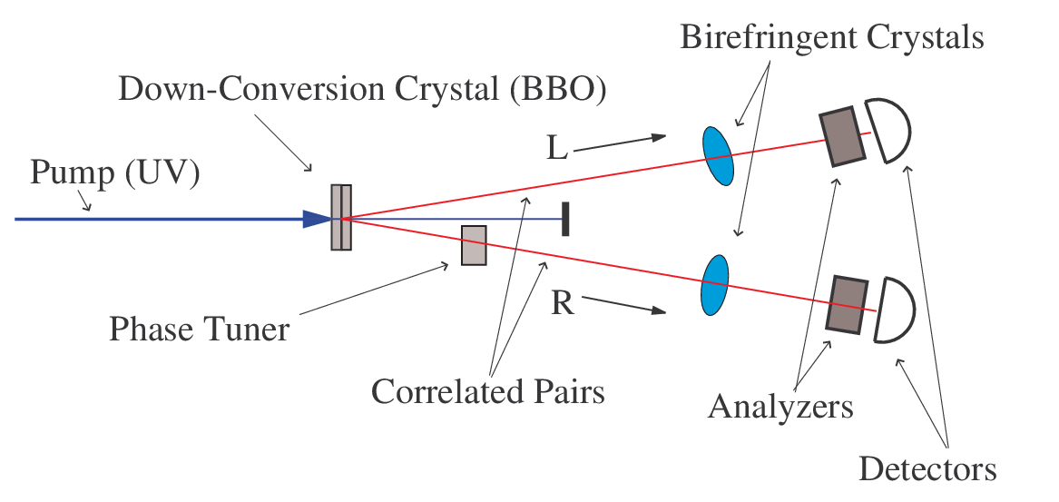
The technique of quantum tomography allows experimental reconstruction of two-photon polarization state density matrices by an appropriate choice of polarization measurements (on members of an ensemble) non-max. With the experimental setup shown in Fig. 10 and using this technique, we compare the theoretical predictions with experimentally observed density matrices. Details of the experiment and results will be reported elsewhere DFS_paper. Here, we simply present the theroetical predictions.
We seek to quantify decoherence properties in a single parameter. To this end, we use the Fidelity of the transmission process, defined here as where () represents the polarization density matrix at the input (output) of the system shumacher. For a mixed input state, we must use mixedFid. A Fidelity of indicates a decoherence-free process. Numerical evaluation of Eq. III.2 allows us to calculate the Fidelity of the transmission process for coupling eigenstates rotated by an arbitrary angle. Such an analysis reveals a Fidelity of 1 for in a birefringent environment with arbitray eigenstates, confirming the prediction that the singlet state is a decoherence-free subspace.
In Fig. 11, we present a graphical representation of the density matrices for each of the four Bell States passing through birefringent crystals in each photon path as calculated from Eq. III.2.
| Input | Output |
|---|---|

| |

| |

| |

|
We see that the singlet state does indeed maintain full coherence in the presence of a unitary frequency-polarization coupling. Since polarization degrees of freedom are analyzed and frequency degrees of freedom are unobserved, such a result demonstrates the robustness of a decoherence-free subspace of two qubits against non-dissipative errors arising from coupling with unutilized (environmental) degrees of freedom.
IV Summary and Conclusions
In summary, we have developed a prescription for calculating density matrices representing one- and two-photon states in the presence of unitary frequency-polarization coupling. With these methods, we have investigated decoherence in quantum systems arising from coupling to unobserved (environmental) degrees of freedom. By inducing frequency-dependent phase errors in photon polarization states and tracing over frequency degrees of freedom, we observe information loss as a particular form of decoherence.
In the one photon case, we applied the results of bang-bang and established the feasibility and utility of “bang-bang” quantum control of decoherence in an optical system. By periodically exchanging the eigenstates of the “environmental” coupling, photon coherence (polarization information) is preserved. We observed this effect in the case in which the strength of the coupling is varied (the “slow-flipping” case); the case in which the basis of the coupling is varied; and the case in which both the basis and the strength of the coupling are varied simultaneously. Additionally, we demonstrated the utility of bang-bang control in the presence of a non-unitary (dissipative) coupling operation. In all cases, we see a qualitative reduction in decoherence for the case in which the quantum control procedure is implemented.
In the two-photon case, we applied general results concerning the existence of decoherence-free subspaces in zanardi; lidar to the case of polarization entangled photon pairs produced in a down-conversion scheme. We found that energy conservation in the down-conversion process gives rise to frequency entanglement which alters the assumptions underlying the prediction of a DFS. In particular, frequency anti-correlation breaks the permutation symmetry of the environmental coupling between opposite photon paths by anti-correlating their respective phase errors. We found that modifying the experimental apparatus to restore the symmetry of the phase errors allows us to produce a truly collective decoherence process, and consequently we recovered the singlet state as a DFS.
In conclusion, we have investigated two procedures for reducing the decoherence of an optical qubit subjected to non-dissipative phase errors and non-unitary dissipative errors. The first procedure, “bang-bang” quantum control, preserves polarization information in a single-photon by rapid, periodic control operations which effectively average out decoherence effects. The second procedure requires entanglement between two photons so that the resulting state exhibits symmetry properties which are immune to collective decoherence. These cases together demonstrate the feasibility of both active and passive protection of coherence properties in an optical qubit.
Appendix A Mathematical Arguments
A.1 Eigenvalues of
Unitarity restricts the possible eigenvalues, , of :
| (48) | |||||
Since is complex with modulus 1, we may write
| (49) |
where is a real-valued function of and , and the subscript refers to polarization mode .
A.2 Operator Relations with and
A.2.1 Proof of Equations 11a, 11b
A.2.2 Derivation of Equations 21a-22b
All four relations follow easily from the definitions of and (Eqs. 9a-9b and 18a-18b). Equation 21a is trivial, since by definition, both operators and act as the identity on . For the other three, we apply the definitions in succession.
| (52) | |||||
| (53) | |||||
| (54) | |||||
| (55) | |||||
Again, if represents a reflection (rotation) we use the upper (lower) sign. From these results, we see that can be treated as a single operator with an associated phase error of . Factoring out the global phase shift of in the last two relations (indicated by the arrow in eqs. 54 and 55), we see that can be treated as a single operator with an associated phase error of .
A.3 Experimental Measures of Coherence
A.3.1 Proof of Equation 26
We begin by defining in Eq. 25 to be an equal superposition of the basis states :
| (56a) | |||||
| (56b) | |||||
Then we have
| (57) | |||||
where indicates the real part.
A.4 Explicit Calculation of Two-Photon Density Matrices
We begin by modeling two-photon density matrices including frequency anti-correlation effects. Substituting the appropriate phase functions (Eq. 41) into Eq. 40, we have an explicit expression for :
| (58) |
We will now calculate assuming the initial state matrix elements, , are given by the density matrix representation of the four Bell States,
| (59) |
In this way, we see the effect of on each of these states. For brevity, let . Then we have,
| (60) | |||||
| (61) |
Note that the dependence on (the variable of integration) drops out of the and terms of so that there is no decoherence due to the frequency distribution of the down-converted photons. However, does not drop out of the and terms of . Due to the finite width of the frequency term , for large , the integral in these terms approaches zero in the same manner as the Fourier integrals of Sect. II.1. Note that the results developed above apply only to decoherence in the basis. The states look different in other bases, so they are subject to decoherence in general.
In order to model decoherence in other bases, and also to model non-collective decoherence, we must include rotation operators in Eq. 58. We define an operator which represents a rotation by in arm L and a rotation by in path R. It can be shown that in the present matrix notation,
| (62) |
It follows that . We can now generalize Eq. 39 by writing the reduced density operator representing polarization degrees of freedom after an input state has passed through crystals of thicknesses and at angles and in the photon paths labeled L and R:
| (63) |
Eq. 63 can be solved numerically given (), the eigenvalues which define .
With the same techniques, we can model density matrices including both frequency and path anti-correlation effects. Substituting the modified phase functions (45) into Eq. III.2, we have an expression which includes both frequency and path anti-correlation effects:
| (64) |
Again, using the four Bell States as input states, we see the effect of on each of these states.
| (65) | |||||
| (66) |
Note that in this case, the dependence on (the variable of integration) drops out of the and terms of . On the other hand, does not drop out of the and terms of . Again, the results developed above apply only to decoherence in the basis. The analytical form of is helpful in developing a physical picture of the decoherence process. In order to calculate the corresponding result for decoherence in an arbitrary basis, we simply set in Eq. 63 and solve numerically. This corresponds to the path anti-correlation procedure described earlier. These results will be presented elsewhere DFS_paper, however, the theoretical predictions are unchanged for the state , since it looks the same in every basis.
Acknowledgements
Experimental and theoretical work was performed in the Quantum Information laboratory of P. G. Kwiat at LANL. We wish to thank A. G. White for his willingness to assist in all stages of this work. At Dartmouth, AJB gratefully acknowledges W. Lawrence and M. Mycek for offering support, advice and feedback at various stages.
References
- (1) W. G. Unruh, Phys. Rev. A51, 992 (1995).
- (2) M. Reck, A. Zeilinger, H. Bernstein, and P. Bertani, Phys. Rev. Lett. 71, 58 (1994).
- (3) N. J. Cerf, C. Adami, and P. G. Kwiat, Phys. Rev. A57, 1479 (1998)
- (4) P. G. Kwiat, J. R. Mitchell, P. D. D. Schwindt, and A. G. White, J. of Mod. Opt. 47, 257 (2000).
- (5) L. Viola, and S. Lloyd, Phys. Rev. A58, 2733 (1998).
- (6) P. Zanardi, Phys. Rev. A56, 4445 (1997).
- (7) D. A. Lidar, I. L. Chuang, and K. B. Whaley, Phys. Rev. Lett. 81, 2594 (1998).
- (8) P. G. Kwiat, K. Mattle, H. Weinfurter, A. Zeilinger, A. Sergienko, and Y. Shih, Phys. Rev. Lett. 75, 4337 (1995).
- (9) P. G. Kwiat, E. Waks, A. G. White, I. Applebaum, and P. Eberhard, Phys. Rev. A60, R773 (1999).
- (10) M. Born, and E. Wolf, Principles of Optics, (Cambridge Univ. Press, Cambridge, 7th Edition, 1999).
- (11) J. J. Sakurai, Modern Quantum Mechanics, Chapter 3, (Addison-Wesley, Massachusetts, 2nd Edition, 1994).
- (12) W. T. Buttler et al., Phys. Rev. Lett. 81, 3283, (1998).
- (13) A. G. White, P. G. Kwiat, D. F. V. James, and P. Eberhard, Phys. Rev. Lett. 83, 3103 (1999).
- (14) L. Mandel, and E. Wolf, Optical Coherence and Quantum Optics, (Cambridge Univ. Press, Cambridge, 1995).
- (15) J. D. Franson, Phys. Rev. A45, 3126 (1992).
- (16) P. G. Kwiat, A. J. Berglund, J. B. Altepeter, and A. G. White, to appear in Science (2000).
- (17) B. Schumacher, Phys. Rev. A51, 2738 (1995).
- (18) R. Jozsa, J. Mod. Optics 41, 2315 (1994).