Encoding a qubit in an oscillatorThanks: CALT-68-2273

Classical information can be carried by either a discrete (digital) signal or a continuous (analog) signal. Although in principle an analog signal can be processed, digital computing is far more robust – a digital signal can be readily re-standardized and protected from damage caused by the gradual accumulation of small errors.

Quantum information can also be carried by either a discrete (finite-dimensional) system like a two-level atom or an electron spin, or by a continuous (infinite-dimensional) system like a harmonic oscillator or a rotor. Even in the finite-dimensional case, quantum information is in a certain sense continuous – a state is a vector in a Hilbert space that can point in any direction. Nevertheless, we have known for nearly five years that cleverly encoded quantum states can be re-standardized and protected from the gradual accumulation of small errors, or from the destructive effects of decoherence due to uncontrolled interactions with the environment [1, 2].

One is tempted to wonder whether we can go still further and protect the quantum state of a system described by continuous quantum variables. Probably this is too much to hope for, since even the problem of protecting analog classical information seems to pose insuperable difficulties.

In this paper we achieve a more modest goal: we describe quantum error-correcting codes that protect a state of a finite-dimensional quantum system (or “qudit”) that is encoded in an infinite-dimensional system. These codes may be useful for implementing quantum computation and quantum communication protocols that use harmonic oscillators or rotors that are experimentally accessible.

We also explain how encoded quantum states can be processed fault tolerantly. Once encoded states have been prepared, a universal set of fault-tolerant quantum gates can be implemented using, in the language of quantum optics, linear optical operations, squeezing, homodyne detection, and photon counting. However, for preparation of the encoded states, nonlinear couplings must be invoked.

Our continuous-variable quantum error-correcting codes are effective in protecting against sufficiently weak diffusive phenomena that cause the position and momentum of an oscillator to drift, or against losses that cause the amplitude of an oscillator to decay. By concatenating with conventional finite-dimensional quantum codes, we can also provide protection against errors that heavily damage a (sufficiently small) subset of all the oscillators in a code block.

A different scheme for realizing robust and efficient quantum computation based on linear optics has been recently proposed by Knill, Laflamme, and Milburn [3, 4].

We begin in §II by describing codes that embed an $n$-state quantum system in a larger $d$-state system, and that protect the encoded quantum information against shifts in the amplitude or phase of the $d$-state system. A realization of this coding scheme based on a charged particle in a magnetic field is discussed in §III. Our continuous-variable codes are obtained in §IV by considering a $d\to\infty$ limit. Formally, the code states of the continuous-variable codes are nonnormalizable states, infinitely squeezed in both position and momentum; in §V we describe the consequences of using more realistic approximate code states that are finitely squeezed. In §VI we outline the theory of more general continuous-variable codes based on lattice sphere packings in higher-dimensional phase space.

We discuss in §VII how continuous-variable codes protect against quantum diffusion, amplitude damping, and unitary errors. In §VIII, we establish a lower bound on the quantum capacity of the Gaussian quantum channel.

We then proceed to develop schemes for fault-tolerant manipulation of encoded quantum information, starting in §IX with a discussion of the symplectic operations that can be implemented with linear optics and squeezing. In §X we discuss the measurement of the error syndrome and error recovery, which can be achieved with symplectic operations and homodyne detection. Completion of the fault-tolerant universal gate set by means of photon counting is described in §XI, and the preparation of encoded states is explained in §XII.

Finally, §XIII contains some further remarks about the physical realization of our coding schemes, and §XIV contains concluding comments.

The main novelty of our new codes is that they are designed to protect against a different type of error than has been considered in previous discussions of quantum coding. This distinction is more easily explained if we first consider not the case of a continuous quantum variable, but instead the (also interesting) case of a “qudit,” a $d$-dimensional quantum system. Quantum codes can be constructed that encode $k$ protected qudits in a block of $N$ qudits, so that the encoded qudits can be perfectly recovered if up to $t$ qudits are damaged, irrespective of the nature of the damage [5, 6, 7, 8]. Error recovery will be effective if errors that act on many qudits at once are rare. More precisely, a general error superoperator acting on $N$ qudits can be expanded in terms of a basis of operators, each of definite “weight” (the number of qudits on which the operator acts nontrivially). Encoded information is well protected if the error superoperator has nearly all its support on operators of weight $t$ or less.

But consider instead a different situation, in which the amplitude for an error to occur on each qudit is not small, but the errors are of a restricted type. The possible errors acting on a single qudit can be expanded in terms of a unitary operator basis with $d^{2}$ elements, the “Pauli operators”:

$$X^{a}Z^{b},\quad a,b=0,1,2,\dots,d-1~.$$

(1)

Here $X$ and $Z$ are generalizations of the Pauli matrices $\sigma_{x}$ and $\sigma_{z}$, which act in a particular basis $\{|j\rangle,j=0,1,2,\dots,d-1\}$ according to

	$\displaystyle X$	$\displaystyle:$	$\displaystyle|j\rangle\rightarrow|j+1~({\rm mod}~d)\rangle~,$
	$\displaystyle Z$	$\displaystyle:$	$\displaystyle|j\rangle\rightarrow\omega^{j}|j\rangle~,$		(2)

where $\omega=\exp(2\pi i/d)$. Note that it follows that

$$ZX=\omega XZ.$$

(3)

For $N$ qudits, there is a unitary operator basis with $d^{2N}$ elements consisting of all tensor products of single-qudit Pauli operators.

We will now imagine that errors with $|a|,|b|$ small compared to $d$ are common, but errors with large $|a|$ and $|b|$ are rare. This type of error model could be expected to apply in the case of a continuous quantum variable, which is formally the $d\rightarrow\infty$ limit of a qudit. For example, decoherence causes the position $q$ and momentum $p$ of a particle to diffuse with some nonzero diffusion constant. In any finite time interval $q$ and $p$ will drift by some amount that may be small, but is certainly not zero. How can we protect encoded quantum information under these conditions?

Fortunately, the general “stabilizer” framework [9, 10] for constructing quantum codes can be adapted to this setting. In this framework, one divides the elements of a unitary operator basis into two disjoint and exhaustive classes: the set ${\cal E}$ of “likely errors” that we want to protect against, and the rest, the “unlikely errors.” A code subspace is constructed as the simultaneous eigenspace of a set of commuting “stabilizer generators,” that generate an Abelian group, the “code stabilizer.” The code can reverse errors in the set ${\cal E}$ if, for each pair of errors $E_{a}$ and $E_{b}$, either $E_{a}^{\dagger}E_{b}$ lies in the stabilizer group, or $E_{a}^{\dagger}E_{b}$ fails to commute with some element of the stabilizer. (In the latter case, the two errors alter the eigenvalues of the generators in distinguishable ways; in the former case they do not, but we can successfully recover from an error of type $a$ by applying either $E_{a}^{\dagger}$ or $E_{b}^{\dagger}$.) In typical discussions of quantum coding, ${\cal E}$ is assumed to be the set of all tensor products of Pauli operators with weight up to $t$ (those that act trivially on all but at most $t$ qudits). But the same principles can be invoked to design codes that protect against errors in a set ${\cal E}$ with other properties.

Quantum codes for continuous variables have been described previously by Braunstein [11] and by Lloyd and Slotine [12]. For example, one code they constructed can be regarded as the continuous limit of a qudit code of the type originally introduced by Shor in the binary ($d=2$) case, an $[[N=9,k=1,2t+1=3]]$ code that protects a single qudit encoded in a block of 9 from arbitrary damage inflicted on any one of the 9. The 8 stabilizer generators of the code can be expressed as

	$\displaystyle Z_{1}Z_{2}^{-1}~,Z_{2}Z_{3}^{-1}~,Z_{4}Z_{5}^{-1}~,Z_{5}Z_{6}^{-1}~,Z_{7}Z_{8}^{-1}~,Z_{8}Z_{9}^{-1}~,$
	$\displaystyle(X_{1}X_{2}X_{3})\cdot(X_{4}X_{5}X_{6})^{-1}~,(X_{4}X_{5}X_{6})\cdot(X_{7}X_{8}X_{9})^{-1}~,$		(4)

and encoded operations that commute with the stabilizer and hence act on the encoded qudit can be chosen to be

	$\displaystyle\bar{Z}$	$\displaystyle=$	$\displaystyle Z_{1}Z_{4}Z_{7}~,$
	$\displaystyle\bar{X}$	$\displaystyle=$	$\displaystyle X_{1}X_{2}X_{3}~.$		(5)

In the $d\rightarrow\infty$ limit, we obtain a code that is the simultaneous eigenspace of eight commuting operators acting on nine particles, which are

	$\displaystyle q_{1}-q_{2}~,q_{2}-q_{3}~,q_{4}-q_{5}~,q_{5}-q_{6}~,q_{7}-q_{8},q_{8}-q_{9}~,$
	$\displaystyle(p_{1}+p_{2}+p_{3})-(p_{4}+p_{5}+p_{6})~,$
	$\displaystyle(p_{4}+p_{5}+p_{6})-(p_{7}+p_{8}+p_{9})~.$		(6)

Logical operators that act in the code space are

	$\displaystyle\bar{q}$	$\displaystyle=$	$\displaystyle q_{1}+q_{4}+q_{7}~,$
	$\displaystyle\bar{p}$	$\displaystyle=$	$\displaystyle p_{1}+p_{2}+p_{3}~.$		(7)

This code is designed to protect against errors in which one of the particles makes a large jump in $q$ or $p$ (or both) while the others hold still. But it provides little protection against small diffusive motions of all the particles, which allow $\bar{q}$ and $\bar{p}$ to drift.

Entanglement purification protocols for continuous variable systems have also been proposed — good entangled states can be distilled from noisy entangled states via a protocol that requires two-way classical communication [13, 14]. These purification protocols work well against certain sorts of errors, but their reliance on two-way classical communication makes them inadequate for accurately preserving unknown states in an imperfect quantum memory, or for robust quantum computation.

Returning to qudits, let us consider an example of a quantum code that can protect against small shifts in both amplitude and phase, but not against large shifts. It is already interesting to discuss the case of a system consisting of a single qudit, but where the dimension $n$ of the encoded system is (of course) less than $d$. For example, a qubit ($n=2$) can be encoded in a system with dimension $d=18$, and protected against shifts by one unit in the amplitude or phase of the qudit; that is, against errors of the form $X^{a}Z^{b}$ where $|a|,|b|\leq 1$. The stabilizer of this code is generated by the two operators

$$X^{6},\quad Z^{6}~,$$

(8)

and the commutation relations of the Pauli operators with these generators are

	$\displaystyle(X^{a}Z^{b})\cdot X^{6}$	$\displaystyle=$	$\displaystyle\omega^{6b}~X^{6}\cdot(X^{a}Z^{b})~,$
	$\displaystyle(X^{a}Z^{b})\cdot Z^{6}$	$\displaystyle=$	$\displaystyle\bar{\omega}^{6a}~Z^{6}\cdot(X^{a}Z^{b})~.$		(9)

Therefore, a Pauli operator commutes with the stabilizer only if $a$ and $b$ are both multiples of $3=18/6$; this property ensures that the code can correct single shifts in both amplitude and phase. Logical operators acting on the encoded qudit are

$$\bar{X}=X^{3}~,\quad\bar{Z}=Z^{3}~,$$

(10)

which evidently commute with the stabilizer and are not contained in it.

Since the codewords are eigenstates of $Z^{6}$ with eigenvalue one, the only allowed values of $j$ are multiples of three. And since there are also eigenstates of $X^{6}$ with eigenvalue one, the codewords are invariant under a shift in $j$ by six units. A basis for the two-dimensional code space is

	$\displaystyle|\bar{0}\rangle={1\over\sqrt{3}}\left(|0\rangle+|6\rangle+|12\rangle\right)~,$
	$\displaystyle|\bar{1}\rangle={1\over\sqrt{3}}\left(|3\rangle+|9\rangle+|15\rangle\right)~.$		(11)

If an amplitude error occurs that shifts $j$ by $\pm 1$, the error can be diagnosed by measuring the stabilizer generator $Z^{6}$, which reveals the value of $j$ modulo 3; the error is corrected by adjusting $j$ to the nearest multiple of 3. Phase errors are shifts in the Fourier transformed conjugate basis, and can be corrected similarly.

This code is actually perfect, meaning that each possible pair of eigenvalues of the generators $X^{6}$ and $Z^{6}$ is a valid syndrome for correcting a shift. There are nine possible errors $\{X^{a}Z^{b},~|a|,|b|\leq 1\}$, and the Hilbert space of the qudit contains nine copies of the two-dimensional code space, one corresponding to each possible error. These “error spaces” just barely fit in the qudit space for $d=18=9\cdot 2$.

Similar perfect codes can be constructed that protect against larger shifts. For $d=r_{1}r_{2}n$, consider the stabilizer generators

$$X^{r_{1}n},\quad Z^{r_{2}n}~.$$

(12)

There is an encoded qunit, acted on by logical operators

	$\displaystyle\bar{X}$	$\displaystyle=$	$\displaystyle X^{r_{1}}~,$
	$\displaystyle\bar{Z}$	$\displaystyle=$	$\displaystyle Z^{r_{2}}~,$		(13)

which evidently commute with the stabilizer and satisfy

$$\bar{Z}\bar{X}=\omega^{r_{1}r_{2}}\bar{X}\bar{Z}=e^{2\pi i/n}\bar{X}\bar{Z}~.$$

(14)

The commutation relations of the Pauli operators with the generators are

	$\displaystyle(X^{a}Z^{b})\cdot X^{r_{1}n}$	$\displaystyle=$	$\displaystyle\omega^{r_{1}nb}~X^{r_{1}n}\cdot(X^{a}Z^{b})$
		$\displaystyle=$	$\displaystyle e^{2\pi ib/r_{2}}~X^{r_{1}n}\cdot(X^{a}Z^{b})~,$
	$\displaystyle(X^{a}Z^{b})\cdot Z^{r_{2}n}$	$\displaystyle=$	$\displaystyle\bar{\omega}^{r_{2}na}~Z^{r_{2}n}\cdot(X^{a}Z^{b})$		(15)
		$\displaystyle=$	$\displaystyle e^{-2\pi ia/r_{1}}~Z^{r_{2}n}\cdot(X^{a}Z^{b})~.$

The phases are trivial only if $a$ is an integer multiple of $r_{1}$ and $b$ an integer multiple of $r_{2}$. Therefore, this code can correct all shifts with

	$\displaystyle|a|$	$\displaystyle<$	$\displaystyle\frac{r_{1}}{2}~,$
	$\displaystyle|b|$	$\displaystyle<$	$\displaystyle\frac{r_{2}}{2}~.$		(16)

The number of possible error syndromes is $r_{1}r_{2}=d/n$, so the code is perfect.

Expressed in terms of $Z$ eigenstates, the codewords contain only values of $j$ that are multiples of $r_{1}$ (since $Z^{r_{2}n}=1$), and are invariant under a shift of $j$ by $r_{1}n$ (since $X^{r_{1}n}=1$). Hence a basis for the $n$-dimensional code subspace is

		$\displaystyle|\bar{0}\rangle$	$\displaystyle={1\over\sqrt{r_{2}}}\left(|0\rangle+|nr_{1}\rangle+\dots+|(r_{2}-1)nr_{1}\rangle\right)~,$		(17)
		$\displaystyle|\bar{1}\rangle$	$\displaystyle={1\over\sqrt{r_{2}}}\left(|r_{1}\rangle+\dots+|((r_{2}-1)n+1)r_{1}\rangle\right)~,$
			$\displaystyle\qquad\qquad\cdot$
			$\displaystyle\qquad\qquad\cdot$
		$\displaystyle|\bar{n}-\bar{1}\rangle$	$\displaystyle={1\over\sqrt{r_{2}}}\left(|(n-1)r_{1}\rangle+\dots+|(r_{2}n-1)r_{1}\rangle\right)~.$

If the states undergo an amplitude shift, the value of $j$ modulo $r_{1}$ is determined by measuring the stabilizer generator $Z^{r_{2}n}$, and the shift can be corrected by adjusting $j$ to the nearest multiple of $r_{1}$. The codewords have a similar form in the Fourier transformed conjugate basis (the basis of $X$ eigenstates), but with $r_{1}$ and $r_{2}$ interchanged. Therefore, amplitude shifts by less than $r_{1}/2$ and phase shifts by less than $r_{2}/2$ can be corrected.

A single electron in a uniform magnetic field in two dimensions provides an enlightening realization of our codes. General translations in a magnetic field are noncommuting, since an electron transported around a closed path acquires an Aharonov-Bohm phase $e^{ie\Phi}$, where $\Phi$ is the magnetic flux enclosed by the path. Two translations $T$ and $S$ commute only if the operator $TST^{-1}S^{-1}$ translates an electron around a path that encloses a flux $\Phi=k\Phi_{0}$, where $\Phi_{0}=2\pi/e$ is the flux quantum and $k$ is an integer.

Translations commute with the Hamiltonian $H$, and two translations $T_{1}$ and $T_{2}$ form a maximally commuting set if they generate a lattice that has a unit cell enclosing one quantum of flux. Simultaneously diagonalizing $H$, $T_{1}$ and $T_{2}$, we obtain a Landau level of degenerate energy eigenstates, one state corresponding to each quantum of magnetic flux. Then $T_{1}$ and $T_{2}^{n}$ are the stabilizer generators of a code, where $\bar{Z}=T_{1}^{1/n}$ and $\bar{X}=T_{2}$ are the logical operators on a code space of dimension $n$.

Suppose the system is in a periodically identified box (a torus), so that $T_{1}^{r_{1}}=(T_{2}^{n})^{r_{2}}=1$ are translations around the cycles of the torus. The number of flux quanta through the torus, and hence the degeneracy of the Landau level, is $nr_{1}r_{2}$. The code, then, embeds an $n$ dimensional system in a system of dimension $d=r_{1}r_{2}n$.

In this situation, the logical operations $\bar{X}$ and $\bar{Z}$ can be visualized as translations of the torus in two different directions; the stabilizer generator $\bar{X}^{n}$ is a translation by a fraction $1/r_{2}$ of the length of the torus in one direction, and the stabilizer generator $\bar{Z}^{n}$ is a translation by $1/r_{1}$ of the length in the other direction. Therefore, for any state in the code space, the wave function of the electron in a cell containing $n$ flux quanta is periodically repeated altogether $r_{1}r_{2}$ times to fill the entire torus. Our code can be regarded as a novel kind of “quantum repetition code” – identical “copies” of the wave function are stored in each of $r_{1}r_{2}$ cells. But of course there is only one electron, so if we detect the electron in one cell its state is destroyed in all the cells.

This picture of the state encoded in a Landau level cautions us about the restrictions on the type of error model that the code can fend off successfully. If the environment strongly probes one of the cells and detects nothing, the wave function is suppressed in that cell. This causes a $\bar{X}$ error in the encoded state with a probability of about $1/2r_{2}$, and a $\bar{Z}$ error with a probability of about $1/2r_{1}$. The code is more effective if the typical errors gently deform the state in each cell, rather than strongly deforming it in one cell.

Formally, we can construct quantum codes for systems described by continuous quantum variables by considering the large-$d$ limit of the shift-resistant codes described in §II. We might have hoped to increase $d$ to infinity while holding $r_{1}/d$ and $r_{2}/d$ fixed, maintaining the ability to correct shifts in both amplitude and phase that are a fixed fraction of the ranges of the qudit. However, since the perfect codes satisfy

$$\frac{r_{1}}{d}=\frac{1}{nr_{2}}~,\quad\frac{r_{2}}{d}=\frac{1}{nr_{1}}~,$$

(18)

this is not possible. Nonetheless, interesting codes can be obtained as the amplitude and phase of the qudit approach the position $q$ and momentum $p$ of a particle – we can hold fixed the size of the shifts $\Delta q$ and $\Delta p$ that can be corrected, as the ranges of $q$ and $p$ become unbounded.

Another option is to take $d\rightarrow\infty$ with $r_{1}/d\equiv\frac{1}{m}$ fixed and $r_{2}=m/n$ fixed, obtaining a rotor $Z=e^{i\theta}$ (or a particle in a periodically identified finite box) that can be protected against finite shifts in both the orientation $\theta$ of the rotor and its (quantized) angular momentum $L$. The stabilizer of this code is generated by

	$\displaystyle Z^{r_{2}n}$	$\displaystyle\rightarrow$	$\displaystyle e^{i\theta m}~,$
	$\displaystyle X^{r_{1}n}$	$\displaystyle=$	$\displaystyle X^{d/r_{2}}\rightarrow e^{-2\pi iL(n/m)}$		(19)

and the logical operations are

	$\displaystyle\bar{Z}$	$\displaystyle=$	$\displaystyle e^{i\theta m/n}$
	$\displaystyle\bar{X}$	$\displaystyle=$	$\displaystyle e^{-2\pi iL/m}$		(20)

Since $\bar{X}$ shifts the value of $\theta$ by $2\pi/m$, and $\bar{Z}$ shifts the value of $L$ by $m/n=r_{2}$, this code can correct shifts in $\theta$ with $\Delta\theta<\pi/m$ and shifts in $L$ with $|\Delta L|<m/2n$.

Alternatively, we can consider a limit in which $r_{1}$ and $r_{2}$ both become large. We may write $r_{1}=\alpha/\varepsilon$ and $r_{2}=1/n\alpha\varepsilon$, where $d=nr_{1}r_{2}=1/\varepsilon^{2}$, obtaining a code with stabilizer generators

	$\displaystyle Z^{r_{2}n}$	$\displaystyle\rightarrow$	$\displaystyle\left(e^{2\pi iq\varepsilon}\right)^{(1/\alpha\varepsilon)}=e^{2\pi iq/\alpha}~,$
	$\displaystyle X^{r_{1}n}$	$\displaystyle\rightarrow$	$\displaystyle\left(e^{-ip\varepsilon}\right)^{(n\alpha/\varepsilon)}=e^{-inp\alpha}~,$		(21)

and logical operations

$$\bar{Z}=e^{2\pi iq/n\alpha}~,\quad\bar{X}=e^{-ip\alpha}~,$$

(22)

where $\alpha$ is an arbitrary real number. Using the identity $e^{A}e^{B}=e^{[A,B]}e^{B}e^{A}$ (which holds if $A$ and $B$ commute with their commutator) and the canonical commutation relation $[q,p]=i$, we verify that

$$\bar{Z}\bar{X}=\omega\bar{X}\bar{Z}~,\quad\omega=e^{2\pi i/n}~.$$

(23)

Since $\bar{X}$ translates $q$ by $\alpha$ and $\bar{Z}$ translates $p$ by $2\pi/n\alpha$, the code protects against shifts with

	$\displaystyle|\Delta q|$	$\displaystyle<$	$\displaystyle\frac{\alpha}{2}~,$
	$\displaystyle|\Delta p|$	$\displaystyle<$	$\displaystyle\frac{\pi}{n\alpha}~.$		(24)

Note that the shifts in momentum and position that the code can correct obey the condition

$$\Delta p\Delta q<{\pi\over 2n}\hbar~.$$

(25)

In typical situations, errors in $q$ and $p$ are of comparable magnitude, and it is best to choose $\alpha=\sqrt{2\pi/n}$ so that

$$\bar{Z}=\exp\left(iq\sqrt{2\pi\over n}\right)~,\quad\bar{X}=\exp\left(-ip\sqrt{2\pi\over n}\right)~.$$

(26)

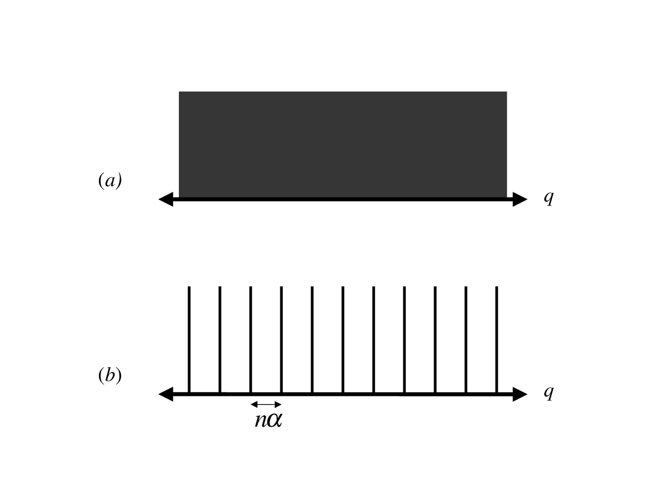
Formally, the codewords are coherent superpositions of infinitely squeezed states, e.g. (up to normalization)

	$\displaystyle|\bar{Z}=\omega^{j}\rangle$	$\displaystyle=$	$\displaystyle\sum_{s=-\infty}^{\infty}|q=\alpha(j+ns)\rangle~,$
	$\displaystyle|\bar{X}=\bar{\omega}^{j}\rangle$	$\displaystyle=$	$\displaystyle\sum_{s=-\infty}^{\infty}|p=\frac{2\pi}{n\alpha}(j+ns)\rangle~.$		(27)

(See Fig. 1.) Of course, realistic codewords will be normalizable finitely squeezed states, rather than nonnormalizable infinitely squeezed states. But squeezing in at least one of $p$ and $q$ is required to comfortably fulfill the condition eq. (25).

The Wigner function associated with the codeword wave function $\psi^{(j)}(q)\equiv\langle q|\bar{Z}=\omega^{j}\rangle$ is a sum of delta functions positioned at the sites of a lattice in phase space, where three quarters of the delta functions are positive and one quarter are negative. Explicitly, we have

	$\displaystyle W^{(j)}(q,p)$	$\displaystyle\equiv$	$\displaystyle{1\over 2\pi}\int_{-\infty}^{\infty}dx~e^{ipx}\psi^{(j)}(q+x/2)^{*}\psi^{(j)}(q-x/2)$		(28)
		$\displaystyle\propto$	$\displaystyle\sum_{s,t=-\infty}^{\infty}(-1)^{st}\delta\left(p-{\pi\over n\alpha}\cdot s\right)$
			$\displaystyle\times~\delta\left(q-\alpha j-{n\alpha\over 2}\cdot t\right)~;$

the delta functions are negative on the sublattice with $s,t$ odd. If we integrate over $p$, the oscillating sign causes the terms with odd $t$ to cancel in the sum over $s$, and the surviving positive delta functions have support at $q=(n\cdot{\rm integer}+j)\alpha$. If we integrate over $q$, the terms with odd $s$ cancel in the sum over $t$, and the surviving positive delta functions have support at $p=(2\pi/n\alpha)\cdot{\rm integer}$. Wigner functions for the $\bar{X}$ eigenstates are similar, but with the roles of $q$ and $p$ interchanged.

It is also of interest to express the encoded states in terms of the basis of coherent states. Consider for example the encoded state with $\bar{X}=1$, which is the unique simultaneous eigenstate with eigenvalue one of the operators $e^{2\pi iq/\alpha}$ and $e^{-ip\alpha}$. In fact starting with any state $|\psi\rangle$, we can construct the encoded state (up to normalization) as

	$\displaystyle\left(\sum_{s=-\infty}^{\infty}e^{-isp\alpha}\right)\cdot\left(\sum_{t=-\infty}^{\infty}e^{2\pi itq/\alpha}\right)|\psi\rangle$
	$\displaystyle=\sum_{s,t}\exp\left[i\left(-sp\alpha+2\pi tq/\alpha+\pi st\right)\right]|\psi\rangle~.$		(29)

In particular, if we choose $|\psi\rangle$ to be the ground state $|0\rangle$ of the oscillator, then the operator $\sum_{s,t}\exp\left[i\left(-sp\alpha+2\pi tq/\alpha+\pi st\right)\right]$ displaces it to a coherent state centered at the point $(q,p)=(s\alpha,2\pi t/\alpha)$ in the quadrature plane. Thus the encoded state is an equally weighted superposition of coherent states, with centers chosen from the sites of a lattice in the quadrature plane whose unit cell has area $2\pi$. Since the coherent states are overcomplete the expansion is not unique; indeed, if we choose $|\psi\rangle$ to be a coherent state rather than the vacuum, then the lattice is rigidly translated, but the encoded state remains invariant.

We can envision the stabilizer of the code as a lattice of translations in phase space that preserve the code words, the lattice generated by the translations $e^{2\pi iq/\alpha}$ and $e^{-inp\alpha}$. In fact, this lattice need not be rectangular – we can encode an $n$-dimensional system in the Hilbert space of a single oscillator by choosing any two variables $Q$ and $P$ that satisfy the canonical commutation relation $[Q,P]=i$, and constructing the code space as the simultaneous eigenstate of $e^{2\pi iQ}$ and $e^{-inP}$. The unit cell of the lattice has area $2\pi\hbar n$, in keeping with the principle that each quantum state “occupies” an area $2\pi\hbar$ in the phase space of a system with one continuous degree of freedom.

Strictly speaking, our codewords are nonnormalizable states, infinitely squeezed in both $q$ and $p$. In practice, we will have to work with approximate codewords that will be finitely squeezed normalizable states. We need to consider how using such approximate codewords will affect the probability of error.

We will replace a position eigenstate $\delta(0)$ by a normalized Gaussian of width $\Delta$ centered at the origin,

	$\displaystyle|\psi_{0}\rangle$	$\displaystyle=$	$\displaystyle\int_{-\infty}^{\infty}{dq\over(\pi\Delta^{2})^{1/4}}e^{-{1\over 2}q^{2}/\Delta^{2}}|q\rangle$		(30)
		$\displaystyle=$	$\displaystyle\int_{-\infty}^{\infty}{dp\over(\pi/\Delta^{2})^{1/4}}e^{-{1\over 2}\Delta^{2}p^{2}}|p\rangle~.$

A codeword, formally a coherent superposition of an infinite number of $\delta$-functions, becomes a sum of Gaussians weighted by a Gaussian envelope function of width $\kappa^{-1}$; in the special case of a two-dimensional code space, the approximate codewords become

	$\displaystyle|\tilde{0}\rangle$	$\displaystyle=$	$\displaystyle N_{0}\sum_{s=-\infty}^{\infty}e^{-{1\over 2}\kappa^{2}(2s\alpha)^{2}}T(2s\alpha)|\psi_{0}\rangle~,$
	$\displaystyle|\tilde{1}\rangle$	$\displaystyle=$	$\displaystyle N_{1}\sum_{s=-\infty}^{\infty}e^{-{1\over 2}\kappa^{2}[(2s+1)\alpha)]^{2}}T[(2s+1)\alpha]|\psi_{0}\rangle~,$		(31)

where $T(a)$ translates $q$ by $a$, $N_{0,1}$ are normalization factors, and we use e.g. $|\tilde{0}\rangle$ rather than $|\bar{0}\rangle$ to denote the approximate codeword. We will assume that $\kappa\alpha$ and $\Delta/\alpha$ are small compared to one, so that $N_{0}\approx N_{1}\approx(4\kappa^{2}\alpha^{2}/\pi)^{1/4}$; then in momentum space, the approximate codeword becomes e.g.,

		$\displaystyle(|\tilde{0}\rangle+|\tilde{1}\rangle)/\sqrt{2}$	$\displaystyle~\approx\left(\kappa^{2}\alpha^{2}\over\pi\right)^{1/4}\int_{-\infty}^{\infty}{dp\over(\pi/\Delta^{2})^{1/4}}e^{-{1\over 2}\Delta^{2}p^{2}}$		(32)
			$\displaystyle\times\sum_{s=-\infty}^{\infty}e^{-{1\over 2}\kappa^{2}(s\alpha)^{2}}e^{ip(\alpha s)}|p\rangle~.$

By applying the Poisson summation formula,

$$\sum_{m=-\infty}^{\infty}e^{-\pi a(m-b)^{2}}=(a)^{-1/2}\sum_{s=-\infty}^{\infty}e^{-\pi s^{2}/a}e^{2\pi isb}~,$$

(33)

this approximate codeword can be rewritten as

		$\displaystyle(|\tilde{0}\rangle+$	$\displaystyle|\tilde{1}\rangle)/\sqrt{2}\approx\left(\kappa^{2}\alpha^{2}\over\pi\right)^{1/4}\int_{-\infty}^{\infty}{dp\over(\pi/\Delta^{2})^{1/4}}e^{-{1\over 2}\Delta^{2}p^{2}}$		(34)
			$\displaystyle\times{\sqrt{2\pi}\over\kappa\alpha}\sum_{m=-\infty}^{\infty}\exp\left[-{1\over 2}\left(p-{2\pi\over\alpha}m\right)^{2}/\kappa^{2}\right]|p\rangle~$
			$\displaystyle=\int_{-\infty}^{\infty}{dp\over(\pi\kappa^{2})^{1/4}}\cdot\left({4\pi\Delta^{2}\over\alpha^{2}}\right)^{1/4}\sum_{m=-\infty}^{\infty}e^{-{1\over 2}\Delta^{2}p^{2}}$
			$\displaystyle\times\exp\left[-{1\over 2}\left(p-{2\pi\over\alpha}m\right)^{2}/\kappa^{2}\right]|p\rangle~,$

again a superposition of Gaussians weighted by a Gaussian envelope. (See Fig. 2.)

The approximate codewords $|\tilde{0}\rangle,|\tilde{1}\rangle$ have a small overlap if $\Delta$ is small compared to $\alpha$ and $\kappa$ is small compared to $\pi/\alpha$. For estimating the error probability caused by the overlap, let’s consider the special case where $q$ and $p$ are treated symmetrically, $\alpha=\sqrt{\pi}$ and $\kappa=\Delta$; then

$$|\langle q|\tilde{0}\rangle|^{2}\approx{2\over\sqrt{\pi}}\sum_{s=-\infty}^{\infty}e^{-4\pi\Delta^{2}s^{2}}\exp[-(q-2s\sqrt{\pi})^{2}/\Delta^{2}]~$$

(35)

and

	$\displaystyle{1\over 2}\left|\langle p|\tilde{0}\rangle+\langle p|\tilde{1}\rangle\right|^{2}$
	$\displaystyle\approx{2\over\sqrt{\pi}}\sum_{m=-\infty}^{\infty}e^{-\Delta^{2}p^{2}}\exp[-(p-2m\sqrt{\pi})^{2}/\Delta^{2}]~.$		(36)

To perform error recovery, we measure the value of $q$ and $p$ modulo $\sqrt{\pi}$ and then correct for the observed shift. In the state $|\tilde{0}\rangle$, the probability of failure is the probability that $q$ is closer to an odd multiple of $\sqrt{\pi}$ than an even multiple, and in the state $(|\tilde{0}\rangle+|\tilde{1}\rangle)/\sqrt{2}$, the error probability is the probability that $p$ is closer to an odd multiple of $\sqrt{\pi}$ than an even multiple. For both the amplitude and phase errors, the intrinsic error probability arising from the imperfections of the approximate codewords becomes exponentially small for small $\Delta$. Using the asymptotic expansion of the error function,

$$\int_{x}^{\infty}dt~e^{-t^{2}}=\left({1\over 2x}\right)e^{-x^{2}}\left(1-O(1/x^{2})\right)~,$$

(37)

we may estimate the error probability by summing the contributions from the tails of all the Gaussians, obtaining

	$\displaystyle{\rm Error~Prob}$	$\displaystyle<$	$\displaystyle{2\over{\sqrt{\pi}}}\left(\sum_{n=-\infty}^{\infty}e^{-4\pi\Delta^{2}n^{2}}\right)\cdot 2\int_{\sqrt{\pi}/2}^{\infty}dq~e^{-q^{2}/\Delta^{2}}$		(38)
		$\displaystyle\sim$	$\displaystyle{2\over\sqrt{\pi}}\cdot{1\over 2\Delta}\cdot 2\Delta\cdot{\Delta\over\sqrt{\pi}}e^{-\pi/4\Delta^{2}}$
		$\displaystyle=$	$\displaystyle{2\Delta\over\pi}e^{-\pi/4\Delta^{2}}~.$

This error probability is about $1\%$ for $\Delta\sim.5$, and is already less than $10^{-6}$ for a still modest value $\Delta\sim.25$. Using finitely squeezed approximate codewords does not badly compromise the error-correcting power of the code, since a gentle spreading in $p$ and $q$ is just the kind of error the code is intended to cope with.

The mean photon number of a finitely squeezed approximate codeword is

$$\langle a^{\dagger}a\rangle+1/2={1\over 2}\langle p^{2}+q^{2}\rangle\approx\Delta^{-2}$$

(39)

for small $\Delta$. Therefore, an error probability of order $10^{-6}$ can be achieved with Gaussian approximate codewords that have mean photon number of about $(.25)^{-2}\sim 16$.

More generally, a finitely squeezed codeword $|\psi\rangle$ can be regarded as a perfect codeword $|\xi\rangle$ that has undergone an error; we may write

$$|\psi\rangle\,=\,\int du\,dv\,\eta(u,v)\,e^{i(-up+vq)}|\xi\rangle,$$

(40)

where $\eta(u,v)$ is an error “wave function.” In the special case of a Gaussian finitely squeezed codeword, we have

$$\eta(u,v)\,=\,\frac{1}{\sqrt{\pi\kappa\Delta}}\exp\Bigl(-\frac{1}{2}(u^{2}/\Delta^{2}+v^{2}/\kappa^{2})\Bigr)~,$$

(41)

where $\Delta$ and $\kappa$ are the squeezing parameters defined above.

If $\eta(u,v)$ vanishes for $|u|>\alpha/2$ or $|v|>\pi/(n\alpha)$, then the error is correctable. In this case, the interpretation of $\eta(u,v)$ as a wave function has a precise meaning, since there is an unambiguous decomposition of a state into codeword and error. Indeed, if $|\xi_{1}\rangle$, $|\xi_{2}\rangle$ are perfect codewords and $|\psi_{1}\rangle$, $|\psi_{2}\rangle$ are the corresponding finitely squeezed codewords with error wave functions $\eta_{1}$, $\eta_{2}$, then

$$\langle\psi_{1}|\psi_{2}\rangle\,=\,\langle\xi_{1}|\xi_{2}\rangle\,\langle\eta_{1}|\eta_{2}\rangle~,$$

(42)

where

$$\langle\eta_{1}|\eta_{2}\rangle=\int du\,dv~\eta_{1}(u,v)^{*}\,\eta_{2}(u,v)~.$$

(43)

The continuous variable codes described in §IV are based on simple lattices in the two-dimensional phase space of a single particle. We can construct more sophisticated codes from lattices in the $(2N)$-dimensional phase space of $N$ particles. Then codes of higher quality can be constructed that take advantage of efficient packings of spheres in higher dimensions.

For a system of $N$ oscillators, a tensor product of Pauli operators can be expressed in terms of the canonical variables $q_{i}$ and $p_{i}$ as

$$U_{\alpha\beta}=\exp\left[i\sqrt{2\pi}\left(\sum_{i=1}^{N}\alpha_{i}p_{i}+\beta_{i}q_{i}\right)\right]~,$$

(44)

where the $\alpha_{i}$’s and $\beta_{i}$’s are real numbers. (In this setting, the Pauli operators are sometimes called “Weyl operators.”) Two such operators commute up to a phase:

$\displaystyle U_{\alpha\beta}U_{\alpha^{\prime}\beta^{\prime}}=e^{2\pi i[\omega(\alpha\beta,\alpha^{\prime}\beta^{\prime})]}U_{\alpha^{\prime}\beta^{\prime}}U_{\alpha\beta}~,$

(45)

where

$$\omega(\alpha\beta,\alpha^{\prime}\beta^{\prime})\equiv\alpha\cdot\beta^{\prime}-\alpha^{\prime}\cdot\beta$$

(46)

is the symplectic form. Thus two Pauli operators commute if and only if their symplectic form is an integer.

Now a general continuous variable stabilizer code is the simultaneous eigenspace of commuting Pauli operators, the code’s stabilizer generators. If the continuous variable phase space is $2N$-dimensional and the code space is a finite-dimensional Hilbert space, then there must be $2N$ independent generators. The elements of the stabilizer group are in one-to-one correspondence with the points of a lattice ${\cal L}$ in phase space, via the relation

$$U(k_{1},k_{2},\dots k_{2N})=\exp\left[i\sqrt{2\pi}\left(\sum_{a=1}^{2N}k_{a}v_{a}\right)\right]~.$$

(47)

Here $\{v_{a},a=1,2,\dots,2N\}$ are the basis vectors of the lattice (each a linear combination of $q$’s and $p$’s), the $k_{a}$’s are arbitrary integers, and $U(k_{1},k_{2},\dots k_{2N})$ is the corresponding element of the stabilizer. For the stabilizer group to be Abelian, the symplectic inner product of any pair of basis vectors must be an integer; that is, the antisymmetric $2N\times 2N$ matrix

$$A_{ab}=\omega(v_{a},v_{b})$$

(48)

has integral entries. The lattice ${\cal L}$ has a $2N\times 2N$ generator matrix $M$ whose rows are the basis vectors,

$$M=\pmatrix{v_{1}\cr v_{2}\cr\cdot\cr\cdot\cr v_{2N}\cr}~.$$

(49)

In terms of $M$, the matrix $A$ can be expressed as

$$A=M\omega M^{T}~,$$

(50)

where $\omega$ denotes the $2N\times 2N$ matrix

$$\omega=\pmatrix{0&I\cr-I&0\cr}~,$$

(51)

and $I$ is the $N\times N$ identity matrix.

The generator matrix of a lattice is not unique. The replacement

$$M\to M^{\prime}=RM$$

(52)

leaves the lattice unmodified, where $R$ is an invertible integral matrix with determinant $\pm 1$ (whose inverse is also integral). Under this replacement, the matrix $A$ changes according to

$$A\to A^{\prime}=RAR^{T}~.$$

(53)

By Gaussian elimination, an $R$ can be constructed such that the antisymmetric matrix $A$ is transformed to

$$A^{\prime}=\pmatrix{0&D\cr-D&0\cr}~,$$

(54)

where $D$ is a positive diagonal $N\times N$ matrix.

There are also Pauli operators that provide a basis for the operations acting on the code subspace – these are the Pauli operators that commute with the stabilizer but are not contained in the stabilizer. The operators that commute with the stabilizer themselves form a lattice ${\cal L}^{\perp}$ that is dual (in the symplectic form) to the stabilizer lattice. The basis vectors of this lattice can be chosen to be $\{u_{b},b=1,2,3,\dots,2N\}$ such that

$$\omega(u_{a},v_{b})=\delta_{ab}~;$$

(55)

then the generator matrix

$$M^{\perp}=\pmatrix{u_{1}\cr u_{2}\cr\cdot\cr\cdot\cr u_{2N}\cr}~$$

(56)

of ${\cal L}^{\perp}$ has the property

$$M^{\perp}\omega M^{T}=I~.$$

(57)

It follows from eq. (48) and eq. (55) that the ${\cal L}$ basis vectors can be expanded in terms of the ${\cal L}^{\perp}$ basis vectors as

$$v_{a}=\sum_{b}~A_{ab}u_{b}~,$$

(58)

or

$$M=AM^{\perp}~,$$

(59)

and hence that

$$\omega(u_{a},u_{b})=\left(A\right)^{-1}_{ba}~,$$

(60)

or

$$M^{\perp}\omega\left(M^{\perp}\right)^{T}=\left(A^{-1}\right)^{T}~.$$

(61)

If the lattice basis vectors are chosen so that $A$ has the standard form eq. (54), then

$$\left(A^{-1}\right)^{T}=\pmatrix{0&D^{-1}\cr-D^{-1}&0\cr}~.$$

(62)

In the special case of a self-dual lattice, corresponding to a code with a one-dimensional code space, both $A$ and $A^{-1}$ must be integral; hence $D=D^{-1}$ and the standard form of $A$ is

$$A=\pmatrix{0&I\cr-I&0\cr}=\omega~.$$

(63)

Since the code subspace is invariant under the translations in ${\cal L}$, we can think of the encoded information as residing on a torus, the unit cell of ${\cal L}$. The encoded Pauli operators $\{\bar{X}^{a}\bar{Z}^{b}\}$ are a lattice of translations on this torus, corresponding to the coset space ${\cal L}^{\perp}/{\cal L}$. The number of encoded Pauli operators is the ratio of the volume of the unit cell of ${\cal L}$ to the volume of the unit cell of ${\cal L}^{\perp}$, namely the determinant of $A$, which is therefore the square of the dimension of the Hilbert space of the code. Thus the dimension of the code space is

$$n=|{\rm Pf}~A|={\rm det}~D~,$$

(64)

where ${\rm Pf}~A$ denotes the Pfaffian, the square root of the determinant of the antisymmetric matrix $A$.

The stabilizer lattice unit cell has volume $|{\rm Pf}~A|$ in units with $h=2\pi\hbar=1$, and the unit cell of the lattice of encoded operations has volume $|{\rm Pf}~A|^{-1}$ in these units. So the code fits an $n$-dimensional code space into $n$ units of phase space volume, as expected.

Codes of the CSS type (those analogous to the binary quantum codes first constructed by Calderbank and Shor [15] and by Steane [16]) are constructed by choosing one lattice ${\cal L}_{q}$ describing stabilizer generators that are linear combinations of the $q$’s, and another lattice ${\cal L}_{p}\subset{\cal L}_{q}^{\perp}$ describing stabilizer generators that are linear combinations of the $p$’s. (Here ${\cal L}_{q}^{\perp}$ denotes the Euclidean dual of the lattice ${\cal L}_{q}$.) The generator matrix of a CSS code has the form

$$M=\pmatrix{M_{q}&0\cr 0&M_{p}}~,$$

(65)

where $M_{q}$ and $M_{p}$ are $N\times N$ matrices, and the integral matrix $A$ has the form

$$A=\pmatrix{0&M_{q}M_{p}^{T}\cr-M_{p}M_{q}^{T}&0\cr}$$

(66)