Wavelets as basis functions in canonical quantization
Abstract
Canonical quantization of electromagnetic field is traditionally done using plane waves. It is possible to formulate the quantization using other complete set of basis functions. Wavelets are a special kind of functions which are localized in real as well as in Fourier space. In this paper we show how wavelets can be used as basis functions in canonical quantization. A countable set of mode functions are obtained. The general formalism of the change of basis is the same for all wavelets which satisfy a multiresolution analysis.
pacs
42.50.-pI INTRODUCTION
Canonical quantization of electromagnetic field is traditionally done using plane waves. The field is enclosed into a cubic cavity and the field operators are expanded using eigenfunctions of the cavity, i.e., plane waves. After quantization it is possible to take the limit of infinite cavity and eliminate the unphysical finite size cavity. The inconvenience of the use of plane waves is that they are delocalized in real space. This makes it difficult to formulate for example photodetection theories. Photodetectors measure the field locally and are sensitive over a finite bandwidth of frequencies. It is possible to use any complete set of basis functions in the quantization [1, 2], so a formulation with a more localized basis functions would be desirable.
The theory of multiresolution analysis (MRA) has been under intensive study during the recent years [3, 4, 5, 6]. A complete set of basis functions in MRA are called wavelets. Wavelets are localized in real as well as in Fourier space. They are parameterized by scale and translation parameters which both get integer values. The translation parameter translates the wavelet in real space. For large negative values of the scale parameter the wavelet is wide and for large scale parameter values narrow. Typical wavelets are orthogonal with respect to both indices. There are many wavelets with different characteristics. Differences include how well wavelets are localized, what kind of Fourier transforms they have, whether they are real or complex and how symmetric they are. It is interesting that some wavelets have compact support, i.e., they are zero outside a certain finite length interval. These kind of wavelets do not have analytical expressions. The main theory of multiresolution analysis is the same for all useful wavelets.
In this paper we show how wavelets can be used as basis functions in the canonical quantization. Real and orthonormal wavelets are used. New mode functions and operators are linear transforms of plane waves and the corresponding operators. Different vector valued mode functions for electric and magnetic fields are obtained. New creation and annihilation operators are the same for both fields and satisfy bosonic commutation relations. This means that formalism of the new operators remains the same and makes it easy to use the new basis. New mode functions are localized and have similar properties as wavelets, for examble they are parameterized by scale and translation parameters.
In Sec. II we give a short introduction to the theory of multiresolution analysis, scaling functions and wavelets. In Sec. III we derive equations for field operators in wavelet basis. In Sec. IV the theory developed in earlier sections is applied to some simple quantum mechanical simulations and the wavelet and plane wave bases are compared. Finally in Sec. V we give our conclusions and suggest several generalizations of the theory developed in this paper.
II Basic properties of scaling functions and wavelets
II.1 Multiresolution analysis and wavelets
In the following we give a brief introduction to the basic properties of wavelets. The discussion follows books [3, 4, 5]. We start with the scaling function , which spans the function space
| (1) |
Introducing a new index by the formula
| (2) |
we can define different function spaces . If is large, , the scaling function is narrow and peaked around some center point. Large negative values gives a function which is wide. The parameter translates the scaling function in a given scale by a factor .
In order to the scaling function to satisfy a multiresolution analysis (MRA) the function space must include the function space with a lower index
| (3) |
When the parameter approaches infinity we get a space of square integrable functions and when approaches minus infinity the result is a null space . Because of multiresolution analysis, it is possible to expand every function in a function space using basis functions of function space . Specifically we can expand scaling functions in using basis functions of . This gives
| (4) |
with some coefficients . We have chosen and used Eq. (2).
The wavelet space is defined to be a difference space between different function spaces spanned by the scaling functions. We define as
| (5) |
Intuitively contains functions which must be added to in order to get . The basis functions in the function space are called wavelets . All functions in can be expanded using translations of a fundamental wavelet, which are obtained using the same equation as for scaling functions, Eq. (2). Because , the wavelet function in can be expanded using scaling functions in . We get
| (6) |
which corresponds to the equation (4) for . The coefficients and are not independent. They satisfy the relation
| (7) |
Using Eq. (3) in Eq. (5) we can decompose the right hand side into subspaces with lower indices. After one iteration we get
| (8) |
We can do the iteration repeatedly and in the infinite limit we get
| (9) |
where has been used. This means that every function which belongs to can be expanded as
| (10) | |||||
The parameter is totally arbitrary. We can take a limit and because the scaling function space can be eliminated giving
| (11) | |||||
i.e., any -function can be expanded using translated and scaled wavelets. In this paper we use only real orthonormal wavelets which have the property
| (12) |
Multiplying Eq. (11) by parts with and integrating we get the coefficients
| (13) |
It follows from the multiresolution analysis that the integral over the wavelet gives zero, i.e.
| (14) |
This means that wavelets must have some kind of oscillating structure as the name suggests.
So far we have not defined any wavelets explicitly. There are several methods to construct wavelets for different purposes. One method is to divide the Fourier space in such a way that the resulting wavelets fulfill multiresolution analysis requirements and are orthogonal. The wavelets obtained using this method can be well localized but do not have a compact support. Another method is to derive wavelets based on the filter coefficients. The filter coefficients of typical wavelets satisfy the fundamental condition
| (15) |
and are orthogonal
| (16) |
If the length of the filter coefficient sequence is long enough these two conditions do not determine the coefficients uniquely. The remaining degrees of freedom can be used to give additional desirable properties to wavelets. Typical choices are to demand the wavelet or scaling function to be as smooth as possible. These kind of wavelets can have a compact support, i.e., they are zero outside a specific region.
II.2 A few examples of wavelets
One of the best known scaling function is a sinc-function
| (17) |
with . The corresponding wavelet is . Figure 1 shows the scaling function and the wavelet which are both localized around . Both functions are not so well localized as would be desirable for many practical applications. The Fourier transforms of the scaling and wavelet functions are
The reason why oscillations do not decay rapidly is because of the abrupt changes of the Fourier transforms at and . One specialty of the sinc-family of wavelets is that the division of frequency space to different scales is orthogonal, i.e., there is no overlap of the Fourier-transforms of wavelets with different scale parameters . Because of poor localization in real space, Shannon wavelets are rarely used.

It is possible to smoothen the change in Fourier transforms in such a way that orthogonality and multiresolution analysis requirements are preserved. The resulting wavelets are called Meyer-wavelets. There are several different Meyer scaling and wavelet functions depending on the smoothening function. The Meyer scaling and wavelet functions used in this paper are shown in Fig. 2. They are clearly more localized than the corresponding Shannon functions. Absolute values of the Fourier transforms of scaling and wavelet functions are shown in Fig. 3. The Fourier transform of a scaling function is flat around . Around frequencies the Fourier transform decays to zero and is zero at larger values. The smoothing compared to Shannon case is clearly seen in both functions. For wavelets two different scales are shown. As parameter increases the transform is wider and shifted further away from the origin.


The length of filter sequences and in Eq. (4) and (6) for sinc and Meyer scaling fuctions and wavelets are infinite. As a result of this wavelets do not have a compact support but are nonzero, although possibly very small, over the whole -axis. It is possible to construct wavelets which have compact support, i.e., they are exactly zero, not just exponentially small, outside a specific region. The length of the filter sequence for these kind of wavelets is finite and the corresponding wavelets and scaling functions do not have analytical forms. One group of these wavelets are the Daubechies wavelets. In this group of wavelets there are several wavelet families which can be characterized by the lengths of filter sequences. As the length of the sequence increases the wavelets and scaling functions become smoother. Figure 4 shows Daubechies scaling and wavelet functions with a filter coefficient length in Eq. (2) and (6). Both functions are nonzero in the interval . They are continuous and derivable. The functions are not symmetric. The general behavior is that the scaling function is concentrated to the left of the nonzero interval and the wavelet is significantly nonzero in the middle.

II.3 Wavelets in higher dimensions
The discussion above has been about one dimensional wavelets. We want to use wavelets as basis functions in canonical quantization so three dimensional wavelets must be used. One method to construct multidimensional wavelets is to use products of one dimensional scaling and wavelet functions [4, 7]. The following products are all wavelets in two dimensions
| (24) | |||||
The integral over all functions above vanishes as is required for wavelets. The two dimensional scaling function is a product of two one dimensional scaling functions
| (25) |
The wavelets with different scaling and translation parameters become
| (26) |
The translation parameter is now a vector with two components which give the translation in and directions. The scaling parameter is a scalar, so scaling is the same in both directions. Note that the scaling of the wavelet is different compared to the one dimensional case. Any two-dimensional -function can be expanded as
| (27) |
Shannon and Meyer wavelets were constructed by dividing the Fourier space. For these wavelets the three different wavelets in two dimensions, obtained by multiplying one dimensional scaling functions and wavelets, are significantly nonzero in different regions of -space. Figure 5 shows nonzero regions for three different wavelets. Wavelets and are nonzero in regions , and , respectively. Wavelet is nonzero in regions , . With a smaller scaling index , the scaling function in the center is split into similar regions with different wavelets. With larger parameter , larger -values are divided to regions. The division of frequency space is exact only for sinc-wavelets. For all other wavelets the Fourier transform has nonzero values also outside of its main region. How well the Fourier transform is localized into the regions depends on the type of a wavelet used. For wavelets with compact support and small filter sequence length the division described above is not very well.

Three dimensional wavelets can be constructed in a similar way as two dimensional ones. We get one scaling function and seven wavelet functions which are products of one dimensional scaling and wavelet functions
| (28) | |||||
The division of -space is a direct generalization of the two dimensional case. The scaling relation becomes
| (29) |
The expansion of -function is given by Eq. (27) with the difference that the -vector is now three dimensional and index gets values from one to seven.
II.4 Expansion of a plane wave using wavelets
In the following section we need expansions of plane waves using wavelets. The normalized plane wave in a box of side can be expanded as
| (30) |
Multiplying by parts with and using orthogonality of wavelets gives the coefficients
| (31) |
The factorization is possible because multidimensional wavelets are products of one dimensional scaling functions and wavelets. The index is either or denoting scaling and wavelet functions respectively. Similar factorization is possible in Eq. (30). Using equation (29) we get after the change of integration variable
| (32) |
Thus every coefficient can be calculated using the translated and scaled Fourier transform of a fundamental wavelet. The scaling parameter changes also the absolute value of the coefficients whereas the translation parameter gives only a phase shift. Because of orthogonality of plane waves and wavelets we get the following relations
| (33) | |||
| (34) |
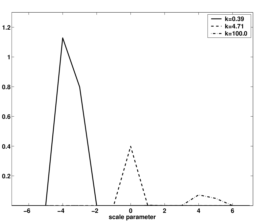
Next we study the parameters more closely. We restrict the discussion to one dimension, i.e., the parameters and are one dimensional. Figure 6 shows the absolute values of the coefficients with several different -values for Meyer wavelets. Note that according to Eq. (31) the translation parameter gives only a phase shift. The coefficients of a plane wave are shown with three different -values. In all cases coefficients with only a few scale parameters are nonzero. For small -values , two scales with parameters have nonzero values. Remember that the Fourier transform of the fundamental () Meyer wavelet is mainly nonzero in the interval . The -value is carefully chosen to be in the middle of the scale interval. It is seen that coefficients for all other -parameters are zero. With large -values the peaks are centered at a higher scale as can be seen from the last peak. Peaks with large scale parameter are smaller than peaks at small scale. This is because of the factor in equation (32). One could think that at large scale the peaks are lower because there are more -values which share the contribution from the single plane wave. Remember that at high scale values the shift of a wavelet is smaller when the translation parameter is changed by one unit.
III Canonical quantization using wavelets
Traditionally canonical quantization of field is done using plane waves as basis functions [1]. The field is enclosed to a cubic of side . All functions can be expanded using the eigenfunctions of the quantization volume, i.e., plane waves. The quantization itself is done by introducing bosonic operators for every basis function. The vector potential of field can be expanded
| (35) |
The vector gives the polarization of the plane wave with wave vector and polarization . Operators and are bosonic annihilation and creation operators. The parameter gets values
| (36) |
For electric and magnetic fields we get
| (37) | |||||
| (38) | |||||
Field operators above are in plane wave basis, which is parameterized by -vectors.
Next we change the basis from plane waves to wavelets. We could just expand the plane waves using wavelets and use this expansion in Eqs. (37) and (38). However this approach would not allow the separation of mode functions and operators. Therefore we proceed by inserting a unity in the form to expansions (37) and (38). The sum is now divided in such a way that all other -values except the operator are changed to . After the use of Eq. (33) for the delta function we get
| (39) | |||||
| (40) | |||||
| (41) | |||||
| (42) |
where the new basis functions and operators are
| (43) | |||||
| (44) | |||||
| (45) |
Similarly for the magnetic field we get
| (46) |
where the operator is given by equation (45) and
| (47) | |||||
| (48) |
The new mode functions behave in the same way as wavelets when the indices are changed. The translation parameter translates the mode functions in three dimensions and the parameter compresses and stretches them. Even though the quantization in the wavelet basis is in free space the operators and mode functions are expanded using a countable set of basis functions. On the contrary to plane waves the polarization of the new mode functions is not constant. As is the case with wavelets, the integral of the mode functions over quantization volume vanishes
| (49) |
This means that also the mode functions have similar ’waviness’ as wavelets.
It is easy to show that the new operators and obey bosonic commutation relations
| (50) | |||
| (51) |
Because of this the operators act like annihilation and creation operators for wavelet modes. This means that the formalism in wavelet basis is the same as with plane wave operators. Multiplying both sides of Eq. (45) by and performing the sum we get with the help of the orthogonality integral
| (52) |
Similarly it is possible to expand plane wave basis functions using wavelet mode functions.
The field Hamiltonian in wavelet basis is obtained as an integral of the energy density over the quantization volume
| (53) |
where expansions (43) and (47) are used for electric and magnetic field operators. In the calculation of (53) the following integrals are needed (last one is listed only for completeness)
| (59) | |||||
where
| (60) |
The identity (59) shows that the coupling constant is a function of the difference of the scaled translation parameters only. Using equations (54) and (55) and the identity
| (61) |
we get after a straightforward calculation for the free field Hamiltonian
| (62) |
The modes are coupled with the coupling constant . The diagonal elements give the energy of the field state which has only one mode with parameters , and excited, i.e., energy of one wavelet quantum. From Eq. (57) and (58) it is seen that the coupling is nonzero only if the corresponding wavelets and Fourier transforms have a nonzero overlap. Because the wavelets are localized both in real and Fourier space this means that for majority of mode pairs the coupling is zero. The detailed structure of the coupling constants depends on the wavelet used. The second term in Eq. (62) is the result of the self-coupling of the modes and gives the zero point energy of the field. As is the case for plane waves the energy per mode is half of the unit excitation field.
IV Numerical simulations using wavelet modes
IV.1 Conventions and wavelets used
In this section we give examples how to apply the theory developed in the last section. We do the calculations in two rather than in three dimensions because visualization is easier and all essential features are included. Thus the -vector is restricted to xy plane and the polarization vector is . Here we exclude the other polarization . The cross product in the expansion of the magnetic field (38) becomes . The choice of the field configuration considered is the same as in our earlier paper [8]. The mode functions for electric and magnetic fields become
| (63) | |||||
| (64) | |||||
where the summation over is now over the xy plane. In the following we choose units such that . In all examples in this section we use the Meyer wavelets shown in Fig. 2. Meyer wavelets were designed using smoothened Fourier transform of Shannon wavelets, so the division of the Fourier-plane shown in Fig. 5 is rather valid. The Fourier transforms of the mode functions are quite similar to the Fourier transforms of the corresponding wavelets. In all simulations the parameters are chosen in such a way that it is necessary to consider only two scales and . This means that the frequencies , and , are excluded. One has to note that in two dimensions the scaling of the wavelet mode functions become
The absolute values of the electric and magnetic mode functions with indices and are shown in Figs. 7 and 8. On the left in both figures there is the mode function with index and on the right . The mode function is the same as case with axes and changed. All mode functions are clearly localized at the origin and have wavelet type of oscillating structure. Because the Fourier transform of two dimensional wavelet is nonzero at higher frequencies than Fourier transforms of and wavelets, the oscillations of mode function have smaller details. As was explained earlier the parameters and scale and translate mode functions.


IV.2 A Gaussian photon
In this section we study a one photon field which is a superposition of different single excitation plane wave modes. The distribution of the absolute values of the mode coefficients is a Gaussian centered at some point with a variance in -space. Thus the field state is
| (66) |
where
| (67) |
The transformation to wavelet basis can be done using the expansion of operators in a wavelet basis (45). The state vector in wavelet basis becomes
| (68) |
where
| (69) |
Because coefficients and factorize, it is possible to factorize the sum (69).
First we briefly study a one dimensional Gaussian distribution. We have a Gaussian photon with parameters , and . The width of the distribution is relatively large so one would expect several scales to have nonzero coefficients. Figure 9 shows coefficients of three different scales as a function of a translation parameter. The peak on the left has the scale parameter . When the translation parameter is changed by one, the wavelet and mode functions are translated by in real space. At scale the translation unit is . The distribution is centered at so coefficients at are centered at . When and the coefficients around and have nonzero values. It is seen that a Gaussian state with the parameters used has the biggest contribution at a scale .

Next we study the time evolution of a two dimensional Gaussian photon. Figure 10 shows the time evolution of the energy density distribution of a photon at two different times. The parameters in Eq. (67) for the initial state at are , , , and . It is seen that the energy density profile of the single excitation field which has a Gaussian distribution in Fourier space is also Gaussian. At a later time the photon has propagated to the right and the intensity profile has spread a little. The time evolution is qualitatively the same as obtained in the paper [8] using plane wave quantization.

On the contrary to plane wave modes the wavelet modes are coupled also for the free field. This makes the operation of the free field Hamiltonian to the statevector, which is needed in the numerical integration, slower. However, most of the coupling constants are zero. Use of this fact makes the operation much faster. The function in the calculation of the coupling coefficients can be used to save memory. In general fewer wavelet mode functions are needed to represent a localized field state than plane wave mode functions.
IV.3 Wavelet mode function initial state
Next we study the time evolution of the field state which at time has only one wavelet mode excited. The mode which is initially excited has parameters , and . The intensity of the field state is shown in Fig. 11. It is clearly localized around which is expected based on the parameters chosen. The Fourier transform for mode function is divided into four parts at the corners of the frequency interval with a specific scaling index , as is explained earlier and shown in Fig. 5. The intensity profile at time is shown in Fig. 11. The intensity is divided to four main parts which all propagate away from the origin. This is understandable based on the Fourier transform of the mode function.

IV.4 Decay of a two level atom
Next we couple a two level atom to the two dimensional field. The interaction Hamiltonian in dipole approximation can be written as
| (70) |
where is the electric dipole moment operator of the two level atom
| (71) |
and the position of the atom. We take the direction of the dipole operator to be in the direction. Using the wavelet expansion of the field (42) we get
| (72) |
In the Hamiltonian the rotating wave approximation (RWA) has been used. The approximation can be done if the mode functions used are well localized in Fourier space. This is the case with Meyer wavelets. The scale parameter determines the frequency interval where the Fourier transform of the mode function is nonzero. Typically the atom interacts with mode functions of only a few, maybe one or two, scales. The mode functions are also spatially localized. Because the interaction is proportional to the electric mode function evaluated at a position of the atom, only mode functions which are centered close to the atom interact with it. In this respect the situation is different compared to the plane wave mode functions which are delocalized. In general the atom is coupled to fewer mode functions than in the plane wave quantization.
Fig. 12 shows the logarithm of the excitation probability of the atom as function of time. The resonance frequency of the atom is and the dipole coupling D=0.06. The atom decays energy to the wavelet modes. The decay is clearly exponential with a decay constant . This corresponds to the theoretical value .

V CONCLUSION
In this paper we have shown how wavelets can be used as basis functions in canonical quantization. Different mode functions for electric and magnetic fields, which are localized both in real and Fourier space, are obtained. Mode functions as well as new operators in wavelet basis are linear transforms of plane wave mode functions and operators. The new annihilation and creation operators satisfy bosonic commutation relations. Because the formalism remains the same, it is easy to change the basis from plane waves to wavelets. We have applied the theory to a few example simulations and showed that the new basis gives well known results in all cases. In this paper we have used wavelet basis for bosonic operators in canonical quantization. The same methods can be used to change basis also for fermionic operators. A localized basis is beneficial for many solid state and semiconductor physics problems.
There are several generalizations and improvements of the theory described in this paper. Complex and biorthogonal wavelets [9] have some benefits compared to real and orthonormal wavelets, for example they can be symmetric. One generalization is to use wavelet packets or multiwavelets instead of wavelets. Finally it would be interesting to compare characteristics of mode functions of different wavelets. It is also possible to construct new wavelets, which have desirable properties, for different problems.
VI ACKNOWLEDGEMENTS
We thank the Academy of Finland (project 43336) for financial support. Computers of the Center for Scientific Computing (CSC) were used in the simulations. The C++ class library ’blitz’ developed by Todd Veldhuizen was used (http://oonumerics.org/blitz/). We thank A. R. Baghai-Wadji, N. Lütkenhaus and K.-A. Suominen for discussions and comments. More figures of different wavelet mode functions can be found from the page http://tftsg6.hip.helsinki.fi/˜mhavukai/wavelets/ .
References
- [1] L. Mandel and E. Wolf, Optical Coherence and Quantum Optics (Cambridge University Press, Cambridge, 1995).
- [2] K. J. Blow, S. J. D. Phoenix, and T. J. Shepherd, Phys. Rev. A 42, 4102 (1990).
- [3] C. S. Burrus, R. A. Gopinath and H. Guo, Introduction to Wavelets and Wavelet Transforms: A Primer (Prentice Hall, Upper Saddle River, New Jersey, 1998).
- [4] J. C. Goswami and A. K. Chan, Fundamentals of Wavelets: Theory, Algorithms and Applications, (John Wiley & sons, New York, 1999).
- [5] C. K. Chui, An Introduction to Wavelets, (Academic Press, San Diego, Calif., 1992).
- [6] I. Daubechies, Ten Lectures on Wavelets, CBMS-NSF, Reg. Conf. Ser. in App. Math. 61, (SIAM, Philadelphia, 1992).
- [7] W. R. Madych in Wavelets - A Tutorial in Theory and Applications (Academic Press, San Diego, Calif.) ed. C. K. Chui, p. 259 (1992).
- [8] M. Havukainen, G. Drobný, S. Stenholm, and V. Bužek, J. Mod. Opt. 46, 1343 (1999).
- [9] A. Cohen, I. Daubechies, and J. C. Feauveau, Comm. of Pure and Appl. Math. 45, 485 (1992)