Quantum algorithm for distributed clock synchronization

Clock synchronization is an important problem with many practical and scientific applications[1, 2]. Accurate timekeeping is at the heart of many modern technologies, including navigation, (the global positioning system), electric power generation (synchronization of generators feeding into national power grids), and telecommunication (synchronous data transfers, financial transactions). Scientifically, clock synchronization is key to projects such as long baseline interferometry (distributed radio telescopes), gravitational wave observation (LIGO), tests of the general theory of relativity, and distributed computation.

The basic problem is easily formulated: determine the time difference $\Delta$ between two spatially separated clocks, using the minimum communication resources. Generally, the accuracy to which $\Delta$ can be determined is a function of the clock frequency stability, and the uncertainty in the delivery times for messages sent between the two clocks. Given the stability of present clocks, and assuming realistic bounded uncertainties in the delivery times (e.g. satellite to ground transmission delays), protocols have been developed which presently allow determination of $\Delta$ to accuracies better than $100$ ns (even for clock separations greater than $8000$ km); it is also predicted that accuracies of $100$ ps should be achievable in the near future.

However, these protocols fail if the message delivery time is too uncertain, because they rely upon the law of large numbers to achieve a constant average delivery time (thus, also requiring $O(2^{2n})$ messages to obtain $n$ digits of $\Delta$). If the required averaging time is longer than the stability time of the local clocks, then these protocols must be replaced. A simple, different, protocol, which succeeds independent of the delivery time, is to just send a clock which keeps track of the delivery time. For example, if Alice mails Bob a wristwatch synchronized to her clock, then when Bob receives it he can clearly calculate the $\Delta$ for their two clocks from the difference between his time and that given by the wristwatch.

This wristwatch protocol is generally impractical, but it suggests another scheme which is intriguing. A quantum bit (qubit) behaves naturally much like a small clock. For example, a nuclear spin in a magnetic field precesses at a frequency given by its gyromagnetic ratio times the magnetic field strength. And an optical qubit, represented by the the presence or absence of a single photon in a given mode, oscillates at the frequency of the electromagnetic carrier. The relative phase between the $|0\rangle$ and $|1\rangle$ states of a qubit thus keeps time, much like a clock, and ticks away during transit. Unlike a classical clock, however, this phase information is lost after measurement, since projection causes the qubit to collapse onto either $|0\rangle$ or $|1\rangle$, so repeated measurements and many qubits are necessary to determine $\Delta$. On the other hand, with present technology it is practical to communicate qubits over long distances through fibers[3, 4], and even in free space[5].

Here, we study this “ticking qubit” protocol for clock synchronization, and establish an upper bound on the number of qubits which must be transmitted in order to determine $\Delta$ to a given accuracy. Surprisingly, we find that only $O(n)$ qubits are needed to obtain $n$ bits of $\Delta$, if we have the freedom of sending qubits which tick at different frequencies. We begin by describing a formal model for this protocol, then the algorithm is presented. Various generalizations and limitations are discussed in the conclusion.

Let $t^{a}$ and $t^{b}$ be the local times on Alice and Bob’s respective clocks. We may assume for now, for the sake of simplicity, that their clocks operate at exactly the same frequency and are perfectly stable. Their goal is to determine the difference $\Delta=t^{b}-t^{a}$, which is initially unknown to either of them. The goal can be accomplished using the following primitive:

We use notation for quantum states and their transforms that is standard in the quantum computation and quantum information community; for an excellent review, see [6]. This can be summarized as follows. $|\psi\rangle$ is the state of a qubit, which can be expressed as a two-component unit vector

$$|\psi\rangle=c_{0}|0\rangle+c_{1}|1\rangle=\left[\begin{array}[]{c}{c_{0}}\\ {c_{1}}\end{array}\right]\,,$$

(1)

where $c_{0}$ and $c_{1}$ are complex numbers satisfying $|c_{0}|^{2}+|c_{1}|^{2}=1$. When measured, a $0$ results, projecting the qubit into the state $|0\rangle$ with probability $|c_{0}|^{2}$; the corresponding happens for $1$.. Operations on qubits are unitary transformations $U$ which are matrices that satisfy $U^{\dagger}U=I$, $U^{\dagger}$ being the complex-conjugate transpose of $U$ and $I$ the identity matrix. For single qubits, any $2$$\times$$2$ unitary transform may be written a rotation operator,

$$e^{i\alpha+i\theta({n}_{x}X+{n}_{y}Y+{n}_{z}Z)/2}\,,$$

(2)

where $\alpha$ specifies a (usually irrelevant) global phase, $X$, $Y$, and $Z$ are the usual Pauli matrices,

$$X=\left[\begin{array}[]{cc}{0}&{1}\\ {1}&{0}\end{array}\right]~~~~~~Y=\left[\begin{array}[]{cc}{0}&{-i}\\ {i}&{0}\end{array}\right]~~~~~~Z=\left[\begin{array}[]{cc}{1}&{0}\\ {0}&{-1}\end{array}\right]\,,$$

(3)

$\hat{n}=[n_{x},n_{y},n_{z}]^{T}$ is a unit real-component vector, and $\theta$ is the rotation angle. Note that $X$, $Y$, and $Z$ themselves are valid unitary operators; simple operations such as these are often called quantum logic gates, and cascading them gives a quantum circuit.

The six stages of the $\mathbf{T}QH(\omega,|\psi\rangle)$ protocol work in the following ways. $\omega$ and $|\psi\rangle$ are inputs, as described in Step 1; we will show below how they can be set usefully. Step 2 follows from the the time-evolution of the qubit during transit. A quantum state $|\psi\rangle$ evolves in time according to the Schrödinger equation

$$-i\hbar\frac{d}{dt}|\psi\rangle={\cal H}|\psi\rangle\,,$$

(4)

where $\cal H$ is the (time-independent) Hamiltonian describing the physical configuration of the system. For example, a spin-$1/2$ particle such as an electron or proton in a magnetic field $B$ has the Hamiltonian ${\cal H}=\hbar\omega Z$, where $\hbar\omega$ is the energy difference between the state of the spin aligned and anti-aligned with $B$. Many other quantum systems, such as a single photon propagating in space, can have a Hamiltonian of this mathematical form. Plugging this $\cal H$ into the solution to the Schrödinger equation,

$$|\psi(t)\rangle=e^{i{\cal H}t/\hbar}|\psi(t=0)\rangle\,,$$

(5)

gives $e^{i\omega t_{12}Z}|\psi\rangle$ after the elapsed time $t_{12}$. Step 3 is true because $t^{b}=t^{a}+\Delta$, and $t_{12}=t^{b}_{2}-t^{b}_{1}=t^{b}_{2}-t^{a}_{1}-\Delta$, so $C_{12}e^{i\omega t_{12}Z}|\psi\rangle=e^{-i\omega Z\Delta}|\psi\rangle$. During the time Bob has the qubit, we assume he’s turned off its evolution, so that although $t^{b}_{4}$ may not equal $t^{b}_{2}$, the qubit does not experience any relative phase shift during that time interval. Step 6 follows because $t_{45}=t^{a}_{5}-t^{a}_{4}=t^{a}_{5}-t^{b}_{4}+\Delta$, and $Xe^{i\theta Z}X=e^{-i\theta Z}$. Summarizing, the net effect of this protocol is to allow Alice to transform a qubit $|\psi\rangle$ into $e^{-2i\omega Z\Delta}|\psi\rangle$.

A simple, but inefficient, algorithm which allows Alice to determine $\Delta$ uses repeated execution of the ticking qubit handshake. She prepares $|\psi\rangle=(|0\rangle+|1\rangle)/\sqrt{2}$, executes $\mathbf{T}QH(\omega,|\psi\rangle)$, and obtains

$$|\psi^{\prime}\rangle=\frac{e^{-2i\omega\Delta}}{\sqrt{2}}|0\rangle+\frac{e^{2i\omega\Delta}}{\sqrt{2}}|1\rangle\,.$$

(6)

She then applies a Hadamard transformation

$$H=\frac{1}{\sqrt{2}}\left[\begin{array}[]{cc}{1}&{1}\\ {1}&{-1}\end{array}\right]$$

(7)

to $|\psi^{\prime}\rangle$, getting

$$\frac{e^{-2i\omega\Delta}+e^{2i\omega\Delta}}{{2}}|0\rangle+\frac{e^{-2i\omega\Delta}-e^{2i\omega\Delta}}{{2}}|1\rangle\,,$$

(8)

such that when she measures the state, a $0$ results with probability $\cos^{2}(2\omega\Delta)$. By the law of large numbers, with high probability, $2^{2n}$ repetitions of this procedure allows Alice to estimate $n$ bits of $\cos^{2}(2\omega\Delta)$, and thus, of $\omega\Delta$. If bounds on the size of $\Delta$ are known in advance, $\omega$ can be chosen wisely to allow $\Delta$ to be determined; otherwise, a few iterations of this procedure with different $\omega$ suffice to initially bound $\Delta$.

This repetition procedure is inefficient because it requires an a number of repetitions exponential in the number of desired digits. It is essentially a classical technique, and is very similar in structure to the usual procedure employed in metrology, Ramsey interferometry[7]. The preparation of $|\psi\rangle$ can be accomplished by applying a Hadamard transformation to $|0\rangle$; this corresponds to the first pulse in the Ramsey scheme. Note, incidentally, that in practice, Hadamard transforms can be replaced with simple $\pi/2$ pulses (operations such as $e^{i\pi Y/4}$), although their introduction here is convenient. The $\mathbf{T}QH$ step corresponds to the free evolution period. And the final Hadamard is the second pulse in Ramsey sequence. It is thus not surprising that repetition is inefficient, since it has the same resource requirements as in Ramsey interferometry.

A much better algorithm, which allows Alice to determine $n$ bits of $\Delta$ using only $O(n)$ repetitions of the ticking qubit handshake, is the following. Alice starts with $m+1$ qubits initialized to $|\phi_{0}\rangle=|0\rangle|0\rangle$, where the decimal base label on the left denotes the $m$ qubit state, and the label on the right, the extra ancillary single qubit. She then applies $m$ Hadamard gates to the $m$ qubits, obtaining

$$|\phi_{1}\rangle=\frac{1}{\sqrt{2^{m}}}\sum_{k=0}^{2^{m}-1}|k\rangle|0\rangle\,.$$

(9)

The first register is now in an equal superposition over all possible states of the $m$ qubits. Next, Alice applies a unitary operation $T$ which does

$$T|k\rangle|0\rangle=|k\rangle e^{2\pi ik\omega\Delta}|0\rangle\,.$$

(10)

This is a nontrivial operation, but assume for now that this is possible and below, we’ll show how this is accomplished. Applying $T$ to $|\phi_{1}\rangle$ gives

$$|\phi_{2}\rangle=\frac{1}{\sqrt{2^{m}}}\sum_{k=0}^{2^{m}-1}e^{2\pi ik\omega\Delta}|k\rangle|0\rangle\,.$$

(11)

Next, Alice applies an inverse quantum Fourier transform $F^{-1}$, which does

$$F^{-1}|k\rangle=\frac{1}{\sqrt{2^{m}}}\sum_{j=0}^{2^{m}-1}e^{-2\pi ijk/2^{m}}|j\rangle\,.$$

(12)

This operation requires only $O(n^{2})$ elementary one and two-qubit gates[8] (in contrast to the classical fast Fourier transform, which requires $O(n2^{n})$ gates to transform an $n$ element vector). This produces the state (dropping the final $|0\rangle$, which is now unimportant)

$$|\phi_{3}\rangle=\frac{1}{2^{m}}\sum_{k=0}^{2^{m}-1}\sum_{j=0}^{2^{m}-1}e^{2\pi ik(\omega\Delta-j/2^{m})}|j\rangle=\sum_{j=0}^{2^{m}-1}c_{j}|j\rangle\,.$$

(13)

$|c_{j}|^{2}$ is clearly peaked around $j=2^{m}\omega\Delta$. If $2^{m}\omega\Delta$ is an integer, then this equality holds, $|c_{j}|^{2}=\delta_{j,\omega\Delta}$, and measuring the first $m$ qubits gives $\omega\Delta$ exactly. Otherwise, it can be shown that if $m=n+\lceil{\log(2+1/2\epsilon)}\rceil$, then measuring the $m$ qubits gives $\omega\Delta$ to $n$ bits of accuracy, with probability of success at least $1-\epsilon$[9, 10].

What we have used in this algorithm is the well-known ability of quantum computation to efficiently determine the eigenvalue of a unitary operator, for a given eigenstate, using a routine known as quantum phase estimation[9, 10]. It is possible to use this subroutine in the present application, clock synchronization, because there can be an efficient implementation of the operator $T$.

Alice can implement $T$ using $m$ calls to $\mathbf{T}QH$. One call is made for each of the $m$ qubits, so we can understand how this works by considering what happens for the $\ell{\rm th}$ qubit. Let $c_{0}|0\rangle+c_{1}|1\rangle$ be the state of this qubit, so that we start with the two-qubit state

$$(c_{0}|0\rangle+c_{1}|1\rangle)|0\rangle\,.$$

(14)

Now apply a controlled-not gate[11], whose transform is described by the unitary matrix

$$\left[\begin{array}[]{cccc}1&0&0&0\\ 0&1&0&0\\ 0&0&0&1\\ 0&0&1&0\end{array}\right]\,,$$

(15)

with the control qubit being the first one. The result is

$$c_{0}|00\rangle+c_{1}|11\rangle\,.$$

(16)

Note how the two qubits are now entangled — this is partially reflected by the fact that if a measurement were performed at this moment on one qubit, the result would completely determine the state of the other qubit. Let $|\psi\rangle$ represent the state of the second qubit; Alice sends this to Bob, performing ${\mathbf{T}QH}(-\pi 2^{\ell-1}\omega,|\psi\rangle)$, Upon completion of that procedure, she is left with the state

$$c_{0}e^{2^{\ell}\pi i\omega\Delta/2}|00\rangle+c_{1}e^{-2^{\ell}\pi i\omega\Delta/2}|11\rangle\,.$$

(17)

She then performs a second controlled-not gate, again with the first qubit as the control, obtaining

	$\displaystyle\left[\rule{0.0pt}{10.33327pt}{c_{0}e^{2^{\ell}\pi i\omega\Delta/2}|0\rangle+c_{1}e^{-2^{\ell}\pi i\omega\Delta/2}|1\rangle}\right]|0\rangle$
	$\displaystyle~~=e^{2^{\ell}\pi i\omega\Delta}\sum_{k_{\ell}}c_{k_{\ell}}|k_{\ell}\rangle e^{2^{\ell}\pi ik_{\ell}\omega\Delta}|0\rangle\,.$		(18)

The $e^{2^{\ell}i\omega\Delta}$ global phase is unobservable, and thus irrelevant to the present calculation and can be dropped. The overall operation $T_{\ell}$ accomplished on this $\ell{\rm th}$ qubit can thus be expressed as

$$T_{\ell}|k_{\ell}\rangle|0\rangle=|k_{\ell}\rangle e^{2^{\ell}\pi ik_{\ell}\omega\Delta}|0\rangle\,,$$

(19)

where $|k_{\ell}\rangle$ represents the $\ell{\rm th}$ qubit. Now, the overall state $|k\rangle$ of the $m$ qubits can be written as $|k\rangle=|k_{0}\rangle|k_{1}\rangle\cdots|k_{m-1}\rangle$, so applying $T=T_{0}T_{1}\cdots T_{m-1}$ gives

	$\displaystyle T|k\rangle|0\rangle=\left[\rule{0.0pt}{10.33327pt}{T_{0}|k_{0}\rangle\,T_{1}|k_{1}\rangle\,\cdots T_{m-1}|k_{m-1}\rangle}\right]|0\rangle$
	$\displaystyle~~=|k\rangle e^{2\pi i\omega\Delta\left({\sum_{\ell}2^{\ell}k_{\ell}}\right)}|0\rangle\,.$		(20)

Since $\sum_{\ell}2^{\ell}k_{\ell}=k$, this construction gives the desired transformation, Eq.(10). Note that the $m$ calls to $\mathbf{T}QH$ can be performed sequentially (as shown in Figure 1), or, by using $m$ ancilla qubits initialized to $|0\rangle$, in parallel, since the algorithm leaves them unchanged.

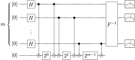
The main caveat to this result is that the tick rate of the qubit $|\psi\rangle$ sent to Bob must span an exponentially large range, from $\sim 1/2\Delta$ to $\sim 2^{m}/\Delta$. If the qubit transmitted in the ${\mathbf{T}QH}$ routine is physically realized by a spin in a magnetic field, this means that there must be “dial settings” for the magnetic field strength which span an exponentially large range. Similarly, if the qubit is represented by a single photon, its carrier must span an exponentially large frequency range. Most critically of all, the stability of the tick rate must be adequate; fluctuations of the magnetic field or index of refraction should be controlled to cause less than roughly a half-wavelength phase shift.

On the other hand, in principle, if it is possible to use a nonlinear optical medium to transport photons between Alice and Bob, then collective photon states whose effective wavelengths can be exponentially short[12] could be used to represent qubits. Furthermore, the shortest wavelength required by the protocol corresponds to the inverse of the accuracy to which $\Delta$ is desired; this means that optical wavelengths roughly correspond to accuracies of fractions of femptoseconds. Time transfer using ground to satellite laser links is under development[13], and photons of other wavelengths, ranging from kilometers to millimeters, are also experimentally feasible. The quantum Fourier transform used in the quantum clock synchronization algorithm is also known to be relatively stable to perturbations[14], and the entire procedure can be further stabilized by using quantum error correction techniques[15, 16, 17, 18].

The quantum algorithm we have described allows two clocks to be synchronized, independent of the uncertainties in message transport time between the clocks, so long as messages are delivered within than the local stability time of the clocks. In its simplest instance, $2^{2n}$ “ticking qubit” communication steps are required to obtain the time difference $\Delta$ to $O(n)$ bits of accuracy. Aside from exponential time, this does not require any demanding physical resources – just the ability to communicate qubits. In the advanced form of the algorithm, only $n$ “ticking qubit” communication steps are required to obtain $O(n)$ bits of $\Delta$, but this procedure requires exponentially demanding physical resources. These results invite further consideration of the problem of clock synchronization with the assistance of quantum resources. For example, it is straightforward to simplify the present protocols to use only one-way communication and no distributed entanglement (these results will be reported in detail elsewhere). It may also be possible to utilize quantum teleportation[19] in a nontrivial manner, but that must be done carefully, since changing the physical form of the qubits usually changes their tick rate; moreover, the two classical bits sent in the teleportation do not tick, and this is not apparently compensated by having an EPR pair around.

We thank Daniel Gottesman and David DiVincenzo for helpful discussions.

References

- [1] B. Simons, J. L. Welch, and N. Lynch, IBM Research Report 6505, (1988).
- [2] W. Lewandowski, J. Azoubib, and W. J. Klepczynski, Proc. IEEE 87, 163 (1999).
- [3] R. J. Hughes et al., Contemp. Phys. 36, 149 (1995), quant-ph/9504002.
- [4] A. Muller, H. Zbinden, and N. Gisin, Europhys. Lett. 33, 334 (1996).
- [5] W. T. Buttler et al., Phys. Rev. A 57, 2379 (1998).
- [6] C. Bennett and D. P. DiVincenzo, Nature 404, 247 (2000).
- [7] J. J. Bollinger, W. M. Itano, D. J. Wineland, and D. J. Heinzen, Phys. Rev. A 54, R4649 (1996).
- [8] D. Coppersmith, IBM Research Report RC 19642 (1994).
- [9] R. Cleve, A. Ekert, C. Macciavello, and M. Mosca, Proc. Roy. Soc. A 454, 339 (1998).
- [10] M. A. Nielsen and I. L. Chuang, Quantum computation and quantum information (Cambridge University Press, Cambridge, UK, 2000).
- [11] A. Barenco et al., Physical Review A 52, 3457 (1995), quant-ph/9503016.
- [12] J. Jacobson, G. Bjork, I. Chuang, and Y. Yamamoto, Physical Review Letters 74, 4835 (1995).
- [13] E. Samain and P. Fridelance, Metrologia 35, 151 (1998).
- [14] A. Barenco, A. Ekert, K. A. Suominen, and P. Torma, Phys. Rev. A 54, 139 (1996).
- [15] A. M. Steane, Physical Review Letters 77, 793 (1996).
- [16] J. Preskill, Proc. Roy. Soc. A: Math., Phys. and Eng. 454, 385 (1998).
- [17] E. Knill and R. Laflamme, Phys. Rev. A 55, 900 (1997), quant-ph/9604034.
- [18] D. Gottesman, Physical Review A 57, 127 (1998), quant-ph/9702029.
- [19] C. H. Bennett et al., Phys. Rev. Lett. 70, 1895 (1993).