Links, Quantum Groups and TQFT’sThanks: This research supported in part by NSF postdoctoral Fellowship #23068

In studying a class of mathematical objects, such as knots, one usually begins by developing ideas and machinery to understand specific features of them. When invariants are discovered, they arise out of such understanding and generally give information about those features. Thus they are often immediately useful for proving theorems, even if they are difficult to compute.

This is not the situation we find ourselves in with the invariants of knots and $3$-manifolds which have appeared since the Jones polynomial. We have a wealth of invariants, all readily computable, but standing decidedly outside the traditions of knot and $3$-manifold theory. They lack a geometric interpretation, and consequently have been of almost no use in answering questions one might have asked before their creation. In effect, we are left looking for the branch of mathematics from which these should have come organically.

In fact, we have an answer of sorts. In [Wit89b], Witten gave a heuristic definition of the Jones polynomial in terms of a topological quantum field theory, following the outline of a program proposed by Atiyah [Ati88]. Specifically, he considered a knot in a $3$-manifold and a connection $A$ on some principal $G$-bundle, with $G$ a simple Lie group. The Chern-Simons functional associates a number $CS(A)$ to $A$, but it is well-defined only up to an integer, so the quantity $\exp(2\pi ikCS(A))$ is well-defined. Also, the holonomy of the connection around the knot is an element of $G$ well-defined up to conjugation, so the trace of it with respect to a given representation is well-defined. Multiplying these two gives a number depending on the knot, the manifold, the representation and the connection. The magic comes when we average over all connections and all principal bundles: Of course, this makes no sense, since there is no apparent measure on the infinite-dimensional space of connections. But proceeding heuristically, such an average should depend only on the manifold, representation and the isotopy type of the knot. Witten argued using a close correspondence with conformal field theory, that when the manifold is $S^{3}$ and the representation the fundamental one, this invariant had combinatorial properties that forced it to be the analogue of the Jones polynomial for the given group (Specifically, the Jones polynomial at certain values of the parameter). Needless to say, a long physics tradition of very successful heuristic reasoning along these lines suggested to Witten that this ill-defined average should make sense in this case.

The fundamental problem of the field, then, is to develop this nonrigorous but beautiful geometric interpretation of the new invariants into a rigorous one that reasonably captures its flavor. This is important for at least two reasons.

First, such an interpretation of the invariants is probably necessary for their application to topological questions. While the invariants have yet to prove themselves in this regard, it is to be hoped that as part of a well-developed theory they could go a long way towards unlocking the mysteries of low-dimensional topology. This theory seems most likely to arise out of something like Witten’s construction, which relates the invariants explicitly to gauge theory and other geometry.

Second, Chern-Simons field theory is a field theory which is clearly nontrivial but which admits an exact combinatorial solution. In this sense, interpreting Witten’s work rigorously is just part of a large endeavor within mathematical physics to understand mathematically the whole of quantum field theory. Such an understanding seems far more tractable for the Chern-Simons theory, with its combinatorial, finite-dimensional expression, than for genuinely physical theories. From this point of view topology may be seen as a laboratory for a particularly simple kind of physics, the understanding of which may point us towards a rigorous foundation for the more complex and physically interesting theories.

Work towards this goal proceeds along two fronts. On the one hand are efforts to understand the geometry and physics of the Chern-Simons field theory, most notably recent efforts to do perturbation theory in this context [AS92, AS94, Kon]. On the other are combinatorial, algebraic, and topological efforts to understand the invariants themselves, especially with an eye towards structures suggested by the physics. This is the subject of the present article.

We begin in Section 1 with a discussion of the Jones polynomial, or more precisely the Kauffman bracket form of it. We mention other invariants, but throughout our focus will be on this example as the easiest. Section 2 first gives a functorial framework for viewing these invariants, constructing the functor explicitly for the Kauffman bracket, and then shows such a functorial setup arises naturally from a certain algebraic structure: a ribbon Hopf algebra. Section 3 discusses quantum groups, the family of ribbon Hopf algebras associated to each Lie algebra. We construct the quantum group associated to $sl_{2}$ explicitly, and show that with the fundamental representation it gives the Kauffman bracket as its invariant.

The last four sections give the construction of the topological quantum field theories. These bear further comment. Witten’s construction obviously gives a $3$-manifold invariant as well, by considering an arbitrary manifold with the empty link. This formed some of the inspiration for Reshetikhin and Turaev’s construction of the $3$-manifold invariants [RT91] using the algebraic machinery of quantum groups. But Atiyah observed that this averaging process (called path integration by physicists), if taken at its word, implied some strong statements about how the invariants behave under cutting and pasting. These statements were formulated by Atiyah into his axioms for a topological quantum field theory, or TQFT [Ati89, Ati90a]. It was shown in [Wal] and [Tur94] that the $3$-manifold invariants satisfy these axioms, although the key ideas of this proof already appeared in [RT91], and in a less rigorous form in [Wit89a, Wit89b]. One of the principal aims of this paper is to give a simple proof of this fact, which is the best rigorous connection we have between these invariants and actual quantum field theory.

Section 4 discusses the properties of the quantum groups at roots of unity, summarized as their being modular Hopf algebras, which allow one to construct TQFT’s from them. Section 5 gives a categorical formulation of TQFT’s. Section 6 sketches a purely combinatorial description of the relevant category, that of biframed $3$-dimensional cobordisms, in terms of surgery on links. This allows us in Section 7 to construct the TQFT out of the link invariants we have already constructed.

This paper is intended to introduce and invite a large mathematical audience to this field. The focus is on giving the flavor and illustrating some of the power of these simple ideas. This is attempted by proving an important result with a minimum of machinery, rather than by surveying the whole of the field, or giving a full account of the machinery. Consequently many interesting areas go unmentioned or barely mentioned. By the same token, the references emphasize pointing the interested reader to good introductory accounts, rather than a thorough assignment of credit. I apologize for any omissions, and point the reader to those same introductory works, many of which have excellent bibliographies, for the complete story.

I would like to thank Scott Axelrod, John Baez, Joan Birman, Dana Fine, Vaughan Jones, Robert Kotiuga, Haynes Miller, Andrew Pressley, Justin Roberts, Lisa Sawin, Isadore Singer, Jim Stasheff, Vladimir Turaev, David Vogan and Eric Weinstein for helpful conversations, comments and suggestions.

The study of knots and links begins with some physics which, while a little eccentric sounding to modern ears, and decidedly wrong, bears a striking resemblance to the physics where this story ends. In 1867 Lord Kelvin proposed that atoms were knotted vortices of ether, and molecules were linked atoms [Kel67]. Efforts began to solve the basic problem of knot theory: When are two knots the same? Early efforts to approach this by careful tabulating and naive searching for invariants failed completely. Modern topology has proved more successful. The approach of focusing exclusively on the knot complement and almost exclusively on its fundamental group has, by dint of great effort, produced a complete but thoroughly impractical algorithm for determining if two prime knots (knots which cannot be cut into two smaller knots) are the same up to orientation of the knot and space [Hem92]. The story for links is more complicated, and not as well understood.

The Jones polynomial, with its descendants, grew from an entirely different branch of mathematics. Its origins bear telling as a study in serendipity, although we will only sketch Jones’ construction, which is buried in the construction in Section 2. Jones, in the course of proving an important result about the ways in which certain algebras of operators sit inside each other [Jon83], constructed an algebra with a trace on it. He then noticed that this algebra gave a representation of the braid group (the mapping-class group of the plane with finitely many points removed). Now by Markov’s theorem [BZ85], links can be represented by elements of the braid group, with two braids giving the same link exactly when they can be connected by conjugation and another move, called stabilization. Any trace is invariant under conjugation, and this particular trace could easily be normalized so as to be invariant under stabilization. Thus presenting the link as a braid, representing the braid in the algebra, and taking the trace gives an invariant of the link. Since the algebra and the trace depend on a parameter $t$, so does the invariant, and it turns out the invariant is essentially a Laurent polynomial in $t$: the celebrated Jones polynomial.

This invariant almost certainly does not come from classical knot theory: It distinguishes links with diffeomorphic complement and detects mirror images for example. It is eminently computable: Although the algorithm is roughly exponential in the number of crossings, and the problem is known to be $\#$P-hard [JVW90], a clever high school student can compute it easily. The collection of these invariants is a fairly good distinguisher of knots, though it does not distinguish all knots, and it is not even known whether it can distinguish a knot from the unknot [Gar]. Maddeningly, these invariants have no geometric interpretation (at least, no rigorous one), and consequently they have provided few purely topological results (chiefly the Tait conjectures, about so-called alternating knots). With such mysteries before us, it is time to do some mathematics.

A link is a smooth embedding of several copies of $S^{1}$ into oriented $S^{3}$. A knot is a link with one component. Links are equivalent if there is an orientation-preserving diffeomorphism of $S^{3}$ taking one to the other. This notion is equivalent to the corresponding PL notion, and to the corresponding topological notion if we restrict to ‘tame’ knots [BZ85]. An oriented link has an orientation on each component, and a framed link comes equipped with a nonzero section of the normal bundle, also up to positive diffeomorphism. We will draw links as in Figure 1, with only transverse-double-point crossings. Oriented links will be drawn with arrows indicating orientation, and framed links will be drawn so that the framing lies in the plane (thus in Figure 1, B represents a different framed knot from A, because the twist cannot be undone). The unknot is the knot which bounds a disk, and has an obvious preferred framing (shown in A). This is all the knot theory we will need to define the Jones polynomial, using a construction due to Kauffman [Kau87].

Let ${\cal L}$ be a projection of a framed, unoriented link $L$. The Kauffman bracket of ${\cal L}$, $\langle{\cal L}\rangle$, is an element of $\mbox{$\mathbb{Z}$}[A,A^{-1}]$, with $A$ an indeterminate, computed by the following skein relations:

(1)		$\displaystyle\langle\phi\rangle$	$\displaystyle=1$
(2)		$\displaystyle\langle\mathchoice{\raisebox{-3.0pt}{ \hskip-1.0pt\psfig{file,height,silent}\hskip 2.0pt}}{\raisebox{-2.0pt}{ \hskip-3.0pt\psfig{file,height,silent}\hskip 2.0pt}}{\raisebox{-2.0pt}{ \hskip-3.0pt\psfig{file,height,silent}\hskip 1.0pt}}{\raisebox{-1.0pt}{ \hskip-1.0pt\psfig{file,height,silent}\hskip 0.0pt}}\rangle$	$\displaystyle=A\langle\mathchoice{\raisebox{-3.0pt}{ \hskip-1.0pt\psfig{file,height,silent}\hskip 2.0pt}}{\raisebox{-2.0pt}{ \hskip-3.0pt\psfig{file,height,silent}\hskip 2.0pt}}{\raisebox{-2.0pt}{ \hskip-3.0pt\psfig{file,height,silent}\hskip 1.0pt}}{\raisebox{-1.0pt}{ \hskip-1.0pt\psfig{file,height,silent}\hskip 0.0pt}}\rangle+A^{-1}\langle\mathchoice{\raisebox{-3.0pt}{ \hskip-1.0pt\psfig{file,height,silent}\hskip 2.0pt}}{\raisebox{-2.0pt}{ \hskip-3.0pt\psfig{file,height,silent}\hskip 2.0pt}}{\raisebox{-2.0pt}{ \hskip-3.0pt\psfig{file,height,silent}\hskip 1.0pt}}{\raisebox{-1.0pt}{ \hskip-1.0pt\psfig{file,height,silent}\hskip 0.0pt}}\rangle$
(3)		$\displaystyle\langle\mathchoice{\raisebox{-3.0pt}{ \hskip-1.0pt\psfig{file,height,silent}\hskip 2.0pt}}{\raisebox{-2.0pt}{ \hskip-3.0pt\psfig{file,height,silent}\hskip 2.0pt}}{\raisebox{-2.0pt}{ \hskip-3.0pt\psfig{file,height,silent}\hskip 1.0pt}}{\raisebox{-1.0pt}{ \hskip-1.0pt\psfig{file,height,silent}\hskip 0.0pt}}\rangle$	$\displaystyle=(-A^{2}-A^{-2})\langle\mathchoice{\raisebox{-3.0pt}{ \hskip-1.0pt\psfig{file,height,silent}\hskip 2.0pt}}{\raisebox{-2.0pt}{ \hskip-3.0pt\psfig{file,height,silent}\hskip 2.0pt}}{\raisebox{-2.0pt}{ \hskip-3.0pt\psfig{file,height,silent}\hskip 1.0pt}}{\raisebox{-1.0pt}{ \hskip-1.0pt\psfig{file,height,silent}\hskip 0.0pt}}\rangle$

where $\phi$ is the link with no components. Equation (2), for example, says that any time you can find three different link projections which look exactly the same except in a small disk, where they look as shown in the equation, then their brackets satisfy this equation. Of course, this means if you happen to know the brackets of the two projections on the right side, this tells you the bracket of the left side. Equation (3) is interpreted similarly, and gives the effect of removing an unlinked unknot from a link.

For example,

	$\displaystyle\langle\mathchoice{\raisebox{-3.0pt}{ \hskip-1.0pt\psfig{file,height,silent}\hskip 2.0pt}}{\raisebox{-2.0pt}{ \hskip-3.0pt\psfig{file,height,silent}\hskip 2.0pt}}{\raisebox{-2.0pt}{ \hskip-3.0pt\psfig{file,height,silent}\hskip 1.0pt}}{\raisebox{-1.0pt}{ \hskip-1.0pt\psfig{file,height,silent}\hskip 0.0pt}}\rangle$	$\displaystyle=A\langle\mathchoice{\raisebox{-3.0pt}{ \hskip-1.0pt\psfig{file,height,silent}\hskip 2.0pt}}{\raisebox{-2.0pt}{ \hskip-3.0pt\psfig{file,height,silent}\hskip 2.0pt}}{\raisebox{-2.0pt}{ \hskip-3.0pt\psfig{file,height,silent}\hskip 1.0pt}}{\raisebox{-1.0pt}{ \hskip-1.0pt\psfig{file,height,silent}\hskip 0.0pt}}\rangle+A^{-1}\langle\mathchoice{\raisebox{-3.0pt}{ \hskip-1.0pt\psfig{file,height,silent}\hskip 2.0pt}}{\raisebox{-2.0pt}{ \hskip-3.0pt\psfig{file,height,silent}\hskip 2.0pt}}{\raisebox{-2.0pt}{ \hskip-3.0pt\psfig{file,height,silent}\hskip 1.0pt}}{\raisebox{-1.0pt}{ \hskip-1.0pt\psfig{file,height,silent}\hskip 0.0pt}}\rangle$
		$\displaystyle=A(-A^{2}-A^{-2})^{2}+A^{-1}(-A^{2}-A^{-2})=-A^{3}(-A^{2}-A^{-2}).$

More generally,

$$\langle\mathchoice{\raisebox{-3.0pt}{ \hskip-1.0pt\psfig{file,height,silent}\hskip 2.0pt}}{\raisebox{-2.0pt}{ \hskip-3.0pt\psfig{file,height,silent}\hskip 2.0pt}}{\raisebox{-2.0pt}{ \hskip-3.0pt\psfig{file,height,silent}\hskip 1.0pt}}{\raisebox{-1.0pt}{ \hskip-1.0pt\psfig{file,height,silent}\hskip 0.0pt}}\rangle=A\langle\mathchoice{\raisebox{-3.0pt}{ \hskip-1.0pt\psfig{file,height,silent}\hskip 2.0pt}}{\raisebox{-2.0pt}{ \hskip-3.0pt\psfig{file,height,silent}\hskip 2.0pt}}{\raisebox{-2.0pt}{ \hskip-3.0pt\psfig{file,height,silent}\hskip 1.0pt}}{\raisebox{-1.0pt}{ \hskip-1.0pt\psfig{file,height,silent}\hskip 0.0pt}}\rangle+A^{-1}\langle\mathchoice{\raisebox{-3.0pt}{ \hskip-1.0pt\psfig{file,height,silent}\hskip 2.0pt}}{\raisebox{-2.0pt}{ \hskip-3.0pt\psfig{file,height,silent}\hskip 2.0pt}}{\raisebox{-2.0pt}{ \hskip-3.0pt\psfig{file,height,silent}\hskip 1.0pt}}{\raisebox{-1.0pt}{ \hskip-1.0pt\psfig{file,height,silent}\hskip 0.0pt}}\rangle=-A^{3}\langle\mathchoice{\raisebox{-3.0pt}{ \hskip-1.0pt\psfig{file,height,silent}\hskip 2.0pt}}{\raisebox{-2.0pt}{ \hskip-3.0pt\psfig{file,height,silent}\hskip 2.0pt}}{\raisebox{-2.0pt}{ \hskip-3.0pt\psfig{file,height,silent}\hskip 1.0pt}}{\raisebox{-1.0pt}{ \hskip-1.0pt\psfig{file,height,silent}\hskip 0.0pt}}\rangle,$$

i.e., adding a twist multiplies any bracket by $-A^{3}$. This is actually a positive twist, corresponding to a clockwise rotation of the framing. A negative twist would multiply the bracket by $-A^{-3}$. The reader can compute that the Kauffman bracket of the right-handed trefoil (C in Figure 1) is $A^{7}+A^{3}+A^{-1}-A^{-9}$.

The point is that the Kauffman bracket does not depend on the projection, but only on the unoriented framed link. This remarkable fact follows from simple calculations, and the framed Reidemeister’s theorem, which says that two projections correspond to the same framed unoriented links if and only if they can be connected by a sequence of a certain finite set of local moves which are roughly Moves I, II, III of Theorem 3 in Section 2 (see [BZ85] for Reidemeister’s theorem, the framed version follows from [Tra83]).

We would like a link invariant, rather than a framed link invariant, if for no other reason than that that is what has been studied since Kelvin (although a case can be made that framed links are a more ‘natural’ object to study: see e.g., Kirby’s theorem in Section 5). We have already seen that adding a positive or negative twist to a link changes the bracket by $-A^{\pm 3}$. It also changes the framing by one full turn. The idea is to correct the bracket so that this move leaves it unchanged, without losing the framed link invariance. To do this, consider an oriented link projection, and label each crossing as positive or negative according to whether it looks like the first or second crossing appearing in Equation (6): I.e., according to whether one strand rotates clockwise or counterclockwise around the other. Then the writhe of an oriented link projection is the number of positive crossings minus the number of negative crossings. For example, the writhe of E in Figure 1 is $+3$, that of F, its mirror image, is $-3$. This is an invariant of oriented framed links, which increases by one when a full twist is added. Thus if ${\cal L}$ is a projection of an oriented link $L$, the quantity

where $\langle{\cal L}\rangle$ is understood to be the bracket of ${\cal L}$ with the orientation removed, depends only on the link $L$.

Even better, notice that in the bracket of the trefoil, exponents increased in steps of four. This is true in general. In fact, a pretty induction on the number of crossing shows that the quantity (4) is an element of $\mbox{$\mathbb{Z}$}[A^{4},A^{-4}]$ if there are an even number of components and is $A^{2}$ times such an element if the number of components is odd. This motivates

One can use Equations (5) and (6) to compute the Jones polynomial more efficiently than via the Kauffman bracket, but it is a bit trickier (see, e.g., [LM88]). We should note that the Jones polynomial as it often appears is our Jones polynomial divided by $-t^{1/2}-t^{-1/2}$, so that its value on the unknot is $1$.

It is worth doing a small computation to see what we have. From the calculations above, the Jones polynomial of the right-handed trefoil, E in Figure 1, is $t^{1/2}(t^{4}-t^{2}-t-1)$. But from the definition, the Jones polynomial of the mirror image of a link (a projection of which is gotten by reversing every crossing of a projection of the link) has the same Jones polynomial, except with $t$ replaced by $t^{-1}$. Thus the left-handed trefoil, F in Figure 1, has invariant $t^{-1/2}(t^{-4}-t^{-2}-t^{-1}-1)$. Since these are different, the two trefoils are not equivalent! Already we can see there is more afoot here than simply the fundamental group of the complement, the major tool of classical knot theory, which must be the same for both. In fact, it was not until 1914 that Dehn proved the inequivalence of these two.

The Jones polynomial was quickly generalized by a host of people [FYH+85, PT87] to a similar, two-variable polynomial, now known as the HOMFLY polynomial (the name, formed from their initials, was unfortunately coined before the work of Przyticki and Traczyk was well known), and by Kauffman to another two-variable polynomial, the Kauffman polynomial, with very similar properties [Kau, Kau87].

Connections with statistical mechanics were quickly noticed [Jon85, Kau88]. Many exactly-solvable statistical mechanical systems had recently been constructed [Bax82] from solutions of the quantum Yang-Baxter Equation (9). Meanwhile, work in inverse scattering theory had found solutions to the classical Yang-Baxter equation associated to Lie algebras [BD82] and efforts to quantize these were just bearing fruit [Dri83, Jim85]. This remarkable confluence resulted in the construction of quantum groups and associated link invariants, which we sketch in the next two sections.

The modern view of algebraic topology is as being about certain functors from the geometric category of topological spaces and homotopy classes of maps, to the algebraic category of groups and homomorphisms. The tremendous success of this program might suggest considering other geometric categories and hoping to find functors from them into algebraic categories. This approach may be taken as the guiding philosophy behind the invariants discussed in this article. In fact, the principal difference between these modern functorial invariants and the classical ones is that here the topological spaces themselves form the morphisms.

In this section we construct the appropriate geometric category, the category of framed tangles [Yet88, Tur89], and show that the Kauffman bracket arises out of a functor from this category to the category of vector spaces. We then show how to construct such a functor from the representation theory of a ribbon Hopf algebra, which we will define. In the next section, we construct the underlying ribbon Hopf algebra, and discuss how to construct a large family of similar ribbon Hopf algebras. Despite the first two paragraphs, this whole section should be accessible to someone knowing little or no category theory.

A tangle is the image of a smooth embedding of a union of circles and intervals into the cylinder $D\times I$, where $D$ is the unit disk in ${\mathbb{C}}$. The intersection of a tangle with the boundary of the cylinder is required to be transverse, to lie in $X\times(\{0\}\cup\{1\})$, where $X$ is the $x$-axis in $D$, and to be exactly the image of the endpoints of the intervals. Tangles are considered up to smooth isotopy of the cylinder leaving $X\times\{0\}$ and $X\times\{1\}$ invariant. Oriented and framed tangles are defined by analogy, but we require the framing to point in the positive $x$ direction at the top and bottom. We define $\operatorname{dom}(T)$ to be the number of intersection points with $X\times\{0\}$, and $\operatorname{codom}(T)$ to be the number of intersection points with $X\times\{1\}$ (for oriented tangles, we must also keep track of the orientations of the points). See Figure 2 for an examples.

Tangles allow two different multiplications. The composition of tangles $T_{1}T_{2}$ is the tangle formed by putting $T_{1}$ on top of $T_{2}$, isotoping so that the boundaries match up smoothly. This is only well-defined if $\operatorname{dom}(T_{1})=\operatorname{codom}(T_{2})$. The tensor product $T_{1}\otimes T_{2}$ is formed by putting them next to each other, and treating them as a single tangle. Both multiplications are associative. See Figure 2 for examples.

In the language of category theory, let $\mathfrak{T}$ be the category whose objects are nonnegative integers, and whose morphisms from $n$ to $m$ are the tangles $T$ with $\operatorname{dom}(T)=n$ and $\operatorname{codom}(T)=m$. Composition is of course composition of tangles. The tensor product makes this category into what is known as a monoidal category. The analogy to keep in mind is the category $\mathfrak{V}$, whose objects are finite-dimensional vector spaces and whose morphisms are linear maps. Here the monoidal structure is given by tensor product of linear maps and vector spaces.

In fact every tangle (hence every link, which is a tangle from the object $0$ to itself) can be constructed out of a handful of generating tangles. Further, we can say exactly which such combinations give the same tangle. This gives a completely algebraic presentation of this monoidal category. The proof of this theorem is not difficult: It involves projections of tangles, and paths between projections.

Much of this structure is quite natural algebraically. Moves VI and VII are just restatements of axioms of a monoidal category. More interestingly, the morphism  , which permutes two objects, looks like the canonical vector space map from $V\otimes W$ to $W\otimes V$, except that its square is not one. The vector space map is an example of a symmetry, a concept arising naturally in category theory (see Section 5). Instead,   and   give the category of tangles a braiding, a weakening of symmetry that comes up in studying 2-categories. In fact, the subcategory of $\mathfrak{T}$ generated by  ,   and   is the free braided, monoidal category generated by one object. This subcategory is none other than the braid group mentioned in Section 1 (actually, the braid groupoid: The endomorphisms of the object $n$ form the mapping class group of the plane with $n$ points removed). The morphisms   and   are like the canonical vector space map from $V\otimes V^{*}$ to ${\mathbb{C}}$ and its dual, and in particular give the category a rigidity or dual structure, also much-studied in category theory. Leaving off Move I entirely (this corresponds to Kauffman’s ‘regular isotopy’ of links) and orienting the tangles we have the free rigid, braided, monoidal category on one object. There are hints that Move I is also natural in the context of $n$-categories [FY89, JS93, KV].

We are looking for a monoidal functor from $\mathfrak{T}$ to $\mathfrak{V}$: That is, an assignment of linear maps to the five generating tangles, such that the seven relations of the previous theorem hold true, with composition interpreted as composition of linear maps and tensor product interpreted as tensor product of linear maps. Call such a map a tangle functor. In particular, a tangle functor would send links to linear maps from ${\mathbb{C}}$ to itself (${\mathbb{C}}$, like the object $0$, is the identity object for tensor multiplication), which are just complex numbers. Thus we get a numerical link invariant.

Hypothesizing that the Kauffman bracket arises from a tangle functor, we see that Equations (2) and (3) are just two more equations that our five linear maps must satisfy. With patience and the additional hint that all of these equations can be satisfied by operators on a two-dimensional space, you would undoubtedly come up with something like the following [Tur89]: Let $V$ be ${\mathbb{C}}^{2}$, and define maps

	$\displaystyle\langle\mathchoice{\raisebox{-3.0pt}{ \hskip-1.0pt\psfig{file,height,silent}\hskip 2.0pt}}{\raisebox{-2.0pt}{ \hskip-3.0pt\psfig{file,height,silent}\hskip 2.0pt}}{\raisebox{-2.0pt}{ \hskip-3.0pt\psfig{file,height,silent}\hskip 1.0pt}}{\raisebox{-1.0pt}{ \hskip-1.0pt\psfig{file,height,silent}\hskip 0.0pt}}\rangle:V\otimes V\to V\otimes V\quad$	$\displaystyle\quad\langle\mathchoice{\raisebox{-3.0pt}{ \hskip-1.0pt\psfig{file,height,silent}\hskip 2.0pt}}{\raisebox{-2.0pt}{ \hskip-3.0pt\psfig{file,height,silent}\hskip 2.0pt}}{\raisebox{-2.0pt}{ \hskip-3.0pt\psfig{file,height,silent}\hskip 1.0pt}}{\raisebox{-1.0pt}{ \hskip-1.0pt\psfig{file,height,silent}\hskip 0.0pt}}\rangle:V\otimes V\to V\otimes V$
	$\displaystyle\langle\mathchoice{\raisebox{-3.0pt}{ \hskip-1.0pt\psfig{file,height,silent}\hskip 2.0pt}}{\raisebox{-2.0pt}{ \hskip-3.0pt\psfig{file,height,silent}\hskip 2.0pt}}{\raisebox{-2.0pt}{ \hskip-3.0pt\psfig{file,height,silent}\hskip 1.0pt}}{\raisebox{-1.0pt}{ \hskip-1.0pt\psfig{file,height,silent}\hskip 0.0pt}}\rangle:V\otimes V\to{\mathbb{C}}\quad\langle\mathchoice{\raisebox{-3.0pt}{ \hskip-1.0pt\psfig{file,height,silent}\hskip 2.0pt}}{\raisebox{-2.0pt}{ \hskip-3.0pt\psfig{file,height,silent}\hskip 2.0pt}}{\raisebox{-2.0pt}{ \hskip-3.0pt\psfig{file,height,silent}\hskip 1.0pt}}{\raisebox{-1.0pt}{ \hskip-1.0pt\psfig{file,height,silent}\hskip 0.0pt}}\rangle:V$	$\displaystyle\to V\quad\langle\mathchoice{\raisebox{-3.0pt}{ \hskip-1.0pt\psfig{file,height,silent}\hskip 2.0pt}}{\raisebox{-2.0pt}{ \hskip-3.0pt\psfig{file,height,silent}\hskip 2.0pt}}{\raisebox{-2.0pt}{ \hskip-3.0pt\psfig{file,height,silent}\hskip 1.0pt}}{\raisebox{-1.0pt}{ \hskip-1.0pt\psfig{file,height,silent}\hskip 0.0pt}}\rangle:{\mathbb{C}}\to V\otimes V$

by the following, writing the basis for $V\otimes V$ as $(1,0)\otimes(1,0)$, $(1,0)\otimes(0,1)$, $(0,1)\otimes(1,0)$, and $(0,1)\otimes(0,1)$:

(7)		$\displaystyle\langle\mathchoice{\raisebox{-3.0pt}{ \hskip-1.0pt\psfig{file,height,silent}\hskip 2.0pt}}{\raisebox{-2.0pt}{ \hskip-3.0pt\psfig{file,height,silent}\hskip 2.0pt}}{\raisebox{-2.0pt}{ \hskip-3.0pt\psfig{file,height,silent}\hskip 1.0pt}}{\raisebox{-1.0pt}{ \hskip-1.0pt\psfig{file,height,silent}\hskip 0.0pt}}\rangle=\begin{bmatrix}A&0&0&0\\ 0&0&A^{-1}&0\\ 0&A^{-1}&A-A^{-3}&0\\ 0&0&0&A\end{bmatrix}\,\,$	$\displaystyle\quad\langle\mathchoice{\raisebox{-3.0pt}{ \hskip-1.0pt\psfig{file,height,silent}\hskip 2.0pt}}{\raisebox{-2.0pt}{ \hskip-3.0pt\psfig{file,height,silent}\hskip 2.0pt}}{\raisebox{-2.0pt}{ \hskip-3.0pt\psfig{file,height,silent}\hskip 1.0pt}}{\raisebox{-1.0pt}{ \hskip-1.0pt\psfig{file,height,silent}\hskip 0.0pt}}\rangle=\begin{bmatrix}A^{-1}&0&0&0\\ 0&A^{-1}-A^{3}&A&0\\ 0&A&0&0\\ 0&0&0&A^{-1}\end{bmatrix}$
(8)		$\displaystyle\langle\mathchoice{\raisebox{-3.0pt}{ \hskip-1.0pt\psfig{file,height,silent}\hskip 2.0pt}}{\raisebox{-2.0pt}{ \hskip-3.0pt\psfig{file,height,silent}\hskip 2.0pt}}{\raisebox{-2.0pt}{ \hskip-3.0pt\psfig{file,height,silent}\hskip 1.0pt}}{\raisebox{-1.0pt}{ \hskip-1.0pt\psfig{file,height,silent}\hskip 0.0pt}}\rangle=\begin{bmatrix}0&A&-A^{-1}&0\end{bmatrix}\quad\langle\mathchoice{\raisebox{-3.0pt}{ \hskip-1.0pt\psfig{file,height,silent}\hskip 2.0pt}}{\raisebox{-2.0pt}{ \hskip-3.0pt\psfig{file,height,silent}\hskip 2.0pt}}{\raisebox{-2.0pt}{ \hskip-3.0pt\psfig{file,height,silent}\hskip 1.0pt}}{\raisebox{-1.0pt}{ \hskip-1.0pt\psfig{file,height,silent}\hskip 0.0pt}}\rangle$	$\displaystyle=\begin{bmatrix}1&0\\ 0&1\end{bmatrix}\quad\langle\mathchoice{\raisebox{-3.0pt}{ \hskip-1.0pt\psfig{file,height,silent}\hskip 2.0pt}}{\raisebox{-2.0pt}{ \hskip-3.0pt\psfig{file,height,silent}\hskip 2.0pt}}{\raisebox{-2.0pt}{ \hskip-3.0pt\psfig{file,height,silent}\hskip 1.0pt}}{\raisebox{-1.0pt}{ \hskip-1.0pt\psfig{file,height,silent}\hskip 0.0pt}}\rangle=\begin{bmatrix}0&-A&A^{-1}&0\end{bmatrix}^{T}.$

The reader can check all the relations with nothing but elementary linear algebra (Moves III and V are best checked by applying Equation (2) first). In particular this confirms that the Kauffman bracket is a framed link invariant. Using the above the Jones polynomial can also be written as a tangle functor.

We now give a set of structures and axioms on an algebra ${\cal A}$ which guarantee that the category whose objects are finite-dimensional representations and whose morphisms are intertwiners (maps between representations commuting with the action of ${\cal A}$) is naturally the range of such a functor. Let us proceed heuristically.

Since sequences of points are sent to a tensor product of representations, the algebra must act on such tensor products. Likewise, it must act on ${\mathbb{C}}$, the image of the object $0$. This requires a bialgebra. That is, an algebra ${\cal A}$, with homomorphisms $\Delta:{\cal A}\to{\cal A}\otimes{\cal A}$ (the coproduct) and $\epsilon:{\cal A}\to{\mathbb{C}}$ (the counit) satisfying

The reason for the terminology is that the adjoint of $\Delta$ together with $\epsilon$ give a multiplication and identity on the dual space, making it an algebra. A bialgebra ${\cal A}$ acts on ${\mathbb{C}}$ by $\epsilon:{\cal A}\to{\mathbb{C}}=\operatorname{End}({\mathbb{C}})$, and if $\rho:{\cal A}\to\operatorname{End}(V)$ and $\tau:{\cal A}\to\operatorname{End}(W)$ are representations, then $(\rho\otimes\tau)\Delta:{\cal A}\to\operatorname{End}(V)\otimes\operatorname{End}(W)$ is a representation on $V\otimes W$.

Now restricting attention to oriented tangles, recall that   and  , with various orientations, were analogous to duality in vector spaces. That is, if a boundary point with one orientation corresponds to a representation $V$, a point with the other orientation should correspond to $V^{*}$, and for example   should correspond to the canonical map from $V^{*}\otimes V$ to ${\mathbb{C}}$. In order for $V^{*}$ to be a representation, our bialgebra ${\cal A}$ must be a Hopf algebra: It should have an antihomomorphism $S:{\cal A}\to{\cal A}$ (antipode) satisfying

where $m$ is the multiplication map. If $\rho:{\cal A}\to\operatorname{End}(V)$ is a representation, then the dual representation $\rho^{*}:{\cal A}\to\operatorname{End}(V^{*})$ is defined by $\rho^{*}(a)v^{*}=v^{*}\circ\rho(S(a))$. The antipode axiom assures that there is a canonical intertwiner from $V\otimes V^{*}$ to the trivial representation. Hopf algebras have a long and distinguished history [Swe69, LR87] outside the scope of this article.

The last piece of information is the braiding  , which should be an intertwiner from $V\otimes W$ to $W\otimes V$. It should not be the flip map, $\sigma_{VW}:v\otimes w\mapsto w\otimes v$, because then we would have $\mathchoice{\raisebox{-3.0pt}{ \hskip-1.0pt\psfig{file,height,silent}\hskip 2.0pt}}{\raisebox{-2.0pt}{ \hskip-3.0pt\psfig{file,height,silent}\hskip 2.0pt}}{\raisebox{-2.0pt}{ \hskip-3.0pt\psfig{file,height,silent}\hskip 1.0pt}}{\raisebox{-1.0pt}{ \hskip-1.0pt\psfig{file,height,silent}\hskip 0.0pt}}=\mathchoice{\raisebox{-3.0pt}{ \hskip-1.0pt\psfig{file,height,silent}\hskip 2.0pt}}{\raisebox{-2.0pt}{ \hskip-3.0pt\psfig{file,height,silent}\hskip 2.0pt}}{\raisebox{-2.0pt}{ \hskip-3.0pt\psfig{file,height,silent}\hskip 1.0pt}}{\raisebox{-1.0pt}{ \hskip-1.0pt\psfig{file,height,silent}\hskip 0.0pt}}$ and our tangle functor would be very uninteresting! The flip map will be an intertwiner whenever ${\cal A}$ is cocommutative, that is, when all $\Delta(a)$ are symmetric. Thus we will expect interesting link invariants only from noncocommutative Hopf algebras. More precisely, if $\Delta^{\prime}(a)=\sigma_{{\cal A}{\cal A}}(\Delta(a))$, then we expect $\Delta\neq\Delta^{\prime}$. They shouldn’t be too different, though, since we want   to behave somewhat like the flip map. It turns out the right notion is for $\Delta$ and $\Delta^{\prime}$ to be connected by an inner automorphism. That is, define a quasitriangular Hopf algebra ${\cal A}$ [Dri85] to be a Hopf algebra ${\cal A}$ together with an invertible element $R\in{\cal A}\otimes{\cal A}$, satisfying

where if $R=\sum_{i}a_{i}\otimes b_{i}$, then $R_{13}=\sum_{i}a_{i}\otimes 1\otimes b_{i}$, $R_{23}=\sum_{i}1\otimes a_{i}\otimes b_{i}$, etc. From these equations one easily gets the Yang-Baxter equation

which will ultimately give us Move III.

Notice cocommutative Hopf algebras are always trivially quasitrangular, with $R=1\otimes 1$. Drinfeld has shown [CP94, 4.2D][Dri87] that one can combine any Hopf algebra ${\cal A}$ with its dual to get a larger Hopf algebra, the ‘quantum double,’ which is quasitriangular (the ones we are interested in are almost of this form). Thus there are lots of them around. They also have a rich and interesting algebraic structure. For example, if we define $u=\sum_{i}S(b_{i})a_{i}$, where $R=\sum_{i}a_{i}\otimes b_{i}$, then

This implies for example that $V$ is isomorphic as a representation to its double dual $V^{**}$, though not by the obvious map.

The representation theory of a quasitriangular Hopf algebra will be a rigid, braided, monoidal category. To get Move I requires a ribbon Hopf algebra [RT90]. The ribbon structure is not as compelling algebraically as the Hopf and quasitriangular structure, perhaps because we do not understand Move I categorically as well as the others. A ribbon Hopf algebra is a quasitriangular Hopf algebra with a grouplike element $G$ (i.e., $\Delta(G)=G\otimes G$ and $\epsilon(G)=1$, hence $S(G)=G^{-1}$) satisfying

Given a representation $(\rho_{V},V)$ and an element $x\in\operatorname{End}(V)$, define the quantum trace $\operatorname{qtr}$ by $\operatorname{qtr}_{V}(x)=\operatorname{tr}(\rho_{V}(G)x)$. The second condition above implies that, identifying $\operatorname{End}(V)$ with $V\otimes V^{*}$, $\operatorname{qtr}$ is the unique to scaling intertwiner from this representation to the trivial one. That $G$ is grouplike means that the quantum trace is additive on direct sums and multiplicative on tensor products. Also important is the quantum dimension of $V$, $\operatorname{qdim}(V)=\operatorname{qtr}_{V}(1)$.

A simple example is called for. Let $G$ be a finite group, and ${\mathbb{C}}G$ be the group algebra. Then the maps

extend by linearity to make ${\mathbb{C}}G$ a cocommutative Hopf algebra. This explains the term grouplike. Being cocommutative, it is a ribbon Hopf algebra with

While these are certainly interesting Hopf algebras, their quasitriangular and ribbon structures are trivial, and we should not expect information about links from them. For that we must wait until the next section.

In putting this together, we see that we have gotten more than we were originally looking for. Specifically, given a ribbon Hopf algebra ${\cal A}$, define a labeled tangle to be an oriented tangle with a finite-dimensional representation of ${\cal A}$ assigned to each component. Thus the domain and codomain are now sequences of oriented points labeled by representations. Assign to such a sequence a representation of ${\cal A}$ by

where $V_{i}$ is a representation, $\varepsilon_{i}$ is $+$ or $-$ indicating the orientation, and $V^{+}_{i}=V_{i}$, $V^{-}_{i}=V_{i}^{*}$.

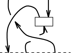
We need to beef up our invariant in a fairly trivial fashion for future sections. Define a ribbon graph exactly as a tangle, except we allow coupons, squares with a definite top, bottom and orientation, with strands allowed to intersect the coupons at distinct points on the top and bottom, as in Figure 3. Theorem 3 is still true of this larger category if we add the coupon as a generator and add relations VIII (and its mirror image) and IX in Figure 3, understood to apply for coupons with any number of incoming and outgoing strands. Given a ribbon Hopf algebra ${\cal A}$, a labeled ribbon graph is one where the strands are labeled by representations of ${\cal A}$ as before, and any coupon with incoming strands labeled $V_{1},\ldots,V_{n}$ and outgoing labeled by $W_{1},\ldots,W_{m}$ is labeled by an intertwiner from $V_{1}\otimes\cdots\otimes V_{n}$ to $W_{1}\otimes\cdots\otimes W_{m}$, with representations replaced by their duals if the corresponding strand is oriented down when it intersects the coupon. It is an easy matter to show that ${\cal F}$ extends to a functor from labeled ribbon graphs to the representation theory of ${\cal A}$, with ${\cal F}$ of a coupon labeled by $f$ being simply $f$. The following summarizes important facts about ${\cal F}$.

Up to this point, this article has been close to being self-contained: All that has been left out are computations, and with a few more precise statements and a sprinkling of hints, the industrious reader could probably reproduce them. I hope also that it has been well-motivated: That the idea of a functor from the tangle category to vector spaces is a natural thing to look for, and that it might reasonably lead one to consider ribbon Hopf algebras. The same will not be true of this section.

It is certainly natural to argue, as we do, that Lie algebras give a nice set of ribbon Hopf algebras which offer trivial link information because they are cocommutative. This suggests deforming them within the set of all ribbon Hopf algebras to get interesting link invariants. If we could argue that there was a unique deformation in the space of ribbon Hopf algebras, or that some sort of quantization described it geometrically, such a construction would seem very natural. Unfortunately, these approaches give only a rough framework in which to proceed, and ultimately one is forced to write down a guess for generators and relations and prove by hand that they give a ribbon Hopf algebra. For this reason we will eschew the deep and significant mathematics in these approaches [CP94, §1-3,6.1,6.2][FT87, Dri83, Dri87], and present the algebras as if by oracle. Likewise, there is a fair amount of interesting technical machinery to prove the basic facts of these algebras [CP94, §6.4,8.1-8.3,10.1][Lus93, Lus88, Ros90a, Jim85, KR88, KR90]: We will merely sketch the easy case $sl_{2}$ and state the broad results in general. Ultimately, from our point of view these quantum groups are a means for extracting geometric information (link invariants) out of quintessentially geometric objects (Lie groups), and it is certainly to be hoped that in the near future we will have a geometric understanding of how they arise.

Recall from the previous section that the group algebra of a finite group is a ribbon Hopf algebra, although the most information it can give about a link is the number of components. It is a little subtle deciding how to define the analogue of the group algebra for a Lie group, but it is clear that morally the same should be true. The best surrogate for this object turns out to be the universal enveloping algebra of the Lie algebra, $U(\mathfrak{g})$. For the group $SL(2)$, this is the algebra $U(sl_{2})$ generated by $\{x,y,h\}$, with relations

where $[a,b]=ab-ba$. Its Hopf algebra structure is determined by

where $a$ is in $\{x,y,h\}$. Its ribbon and quasitriangular structure is trivial, $R=1\otimes 1$ and $G=1$. The universal enveloping algebras of the other simple Lie algebras have similar, if more complicated presentations [Hum72]. Given such a Lie algebra $\mathfrak{g}$, there is associated an algebra $U_{s}(\mathfrak{g})$, the quantum universal enveloping algebra of $\mathfrak{g}$, depending on a nonzero complex parameter $s$. It will prove to be a ribbon Hopf algebra, and in an appropriate sense will approach $U(\mathfrak{g})$ as a ribbon Hopf algebra as $s\to 1$. These quantized universal enveloping algebras are collectively called quantum groups, though the term is sometimes used more generally to refer to ribbon Hopf algebras, quasitriangular Hopf algebras, or even all Hopf algebras.

$U_{s}(sl_{2})$ is the algebra generated by $\{x,y,h\}$ subject to the relations

There are a number of artifices for interpreting the last equation, none entirely satisfactory (the casual reader is encouraged to ignore the problem). Ours is as follows: Let $U(sl_{2})^{\prime}$ be the completion of $U(sl_{2})$ in the topology of convergence on every finite-dimensional representation, and let the closure of the subalgebra generated by $h$ be ${\cal H}$. Notice the right side of the last equation is in ${\cal H}$ for all $s\neq 0$, because every finite-dimensional representation is spanned by eigenvectors of $h$ with integer eigenvalues. Consider the algebra spanned by free products of $x$, $y$ and elements of ${\cal H}$, with the topology inherited from ${\cal H}$. The above equations generate an ideal in this algebra, and the quotient by the closure of that ideal is the algebra $U_{s}(sl_{2})$.

This algebra is really just $U(sl_{2})$ in disguise. Specifically, if we use $\bar{x}$, $\bar{y}$, $\bar{h}$ temporarily to denote the generators of $U(sl_{2})$ and recall that the Casimir element is $C=(\bar{h}+1)^{2}/4+\bar{y}\bar{x},$ then the map $\varphi:U_{s}(sl_{2})\to U(sl_{2})^{\prime}$ given by

is a homomorphism for all $s\neq 0$. Further, this homomorphism is 1-1 and has dense range if $s$ is not a root of unity (essentially because the coefficient of $\bar{x}$ is invertible) [CP94, §4.6][Jim85]. Thus up to completions $U_{s}(sl_{2})$ and $U(sl_{2})$ are isomorphic as algebras. So $U_{s}(sl_{2})$ is semisimple, its finite-dimensional representations are in one to one correspondence with that of $U(sl_{2})$, and the actions of $h$ and $\bar{h}$ on these representations are the same. In particular, they have the same formal characters.

The Hopf algebra structure is given by

and the rest as in the $U(sl_{2})$ case. The key observation is that these maps commute with the operator $[h,\cdot]$. From this and the fact that the formal characters are the same as for $U(sl_{2})$ it is easy to see that duals of representations and decomposition of tensor products into irreducible representations are the same (away from a root of unity) as in the classical case.

The quasitriangular structure is quite a bit trickier. Define quantum integers

Then

The infinite sum is well defined in the usual topology, because only finitely many terms are nonzero on any given pair of representations.

If you believe that all the axioms of a ribbon Hopf algebra are satisfied by the algebra above, you should be wondering what the tangle functor looks like. First we must understand the representation theory explicitly. For this recall that $sl_{2}$ has an $n$-dimensional representation for each $n>0$, with basis $\{v_{i}\}_{i=1}^{n}$ such that

and that the action of $h$ is independent of $s$ (by the isomorphism). It is easy to reconstruct the representation $V_{n}$ of $U_{s}(sl_{2})$ with basis $\{v_{i}\}_{i=1}^{n}$ such that

It is now easy to compute the action of $R$ on $V_{2}\otimes V_{2}$, and composing with the flip map gives

$$\mathchoice{\raisebox{-3.0pt}{ \hskip-1.0pt\psfig{file,height,silent}\hskip 2.0pt}}{\raisebox{-2.0pt}{ \hskip-3.0pt\psfig{file,height,silent}\hskip 2.0pt}}{\raisebox{-2.0pt}{ \hskip-3.0pt\psfig{file,height,silent}\hskip 1.0pt}}{\raisebox{-1.0pt}{ \hskip-1.0pt\psfig{file,height,silent}\hskip 0.0pt}}\to\begin{bmatrix}s&0&0&0\\ 0&0&s^{-1}&0\\ 0&s^{-1}&s-s^{-3}&0\\ 0&0&0&s\end{bmatrix}.$$

Identifying $V$ with $V^{*}$ by the intertwiner $\alpha:v_{1}\mapsto sv_{2}^{*}$, $\alpha:v_{2}\mapsto-s^{-1}v_{1}^{*}$ gives

$$\mathchoice{\raisebox{-3.0pt}{ \hskip-1.0pt\psfig{file,height,silent}\hskip 2.0pt}}{\raisebox{-2.0pt}{ \hskip-3.0pt\psfig{file,height,silent}\hskip 2.0pt}}{\raisebox{-2.0pt}{ \hskip-3.0pt\psfig{file,height,silent}\hskip 1.0pt}}{\raisebox{-1.0pt}{ \hskip-1.0pt\psfig{file,height,silent}\hskip 0.0pt}}=\begin{bmatrix}0&-s&s^{-1}&0\end{bmatrix}\qquad\mathchoice{\raisebox{-3.0pt}{ \hskip-1.0pt\psfig{file,height,silent}\hskip 2.0pt}}{\raisebox{-2.0pt}{ \hskip-3.0pt\psfig{file,height,silent}\hskip 2.0pt}}{\raisebox{-2.0pt}{ \hskip-3.0pt\psfig{file,height,silent}\hskip 1.0pt}}{\raisebox{-1.0pt}{ \hskip-1.0pt\psfig{file,height,silent}\hskip 0.0pt}}=\begin{bmatrix}0&s&-s^{-1}&0\end{bmatrix}$$

with the other generating tangles determined by these. Notice this is almost an unoriented tangle functor—in fact the Kauffman bracket functor, Equations (7) and (8), with $A=s$—except for an annoying minus sign in  . The link invariant will actually be the Kauffman bracket times $(-1)^{w}$, where $w$ is the total winding number of the link projection ($(-1)^{w}$ is a framed, unoriented link invariant!). In general any irreducible self-dual representation gives, on choosing such an $\alpha$, either an unoriented functor or a functor which differs from one by a minus sign in  . Kirillov and Reshetikhin [KR88] nicely fix this problem for $sl_{2}$ by constructing $U_{q}(sl_{2})$ as a deformation of $U(sl_{2})$ with a nonstandard quasitriangular (really triangular) structure.

We have only described the functor with everything labeled by the two-dimensional representation, but we have really constructed much more than that. There is enough information above to write down the full theory for all representations, but no neat skein-theory description has been found for the corresponding invariant.

It is now clearer where the skein relation in Equation (2) is coming from. $V_{2}\otimes V_{2}$ breaks up as the sum of two irreducible representations, the trivial one and $V_{3}$, and thus the space of intertwiners on it is two-dimensional. The two fragments pictured on the right side of Equation (2), interpreted as tangles, correspond to the identity intertwiner and a multiple of the projection onto the trivial subrepresentation. They span the space of intertwiners, which includes  .

As for other Lie algebras, the story is essentially the same. A similar, but more complicated presentation of $U_{s}(\mathfrak{g})$ can be given, and shown in the same sense to be isomorphic to $U(\mathfrak{g})$ (though in general the isomorphism does not admit explicit formulae as in the $sl_{2}$ case). The ribbon Hopf structure can all be written down explicitly, and the representation theory is ‘the same’ as for the original Lie algebra except at roots of unity [CP94, §8.3,10.1]. The link invariants coming from the fundamental representation of $sl_{n}$ are particular values of the two-variable HOMFLY polynomial. The polynomials for $B_{n}$, $C_{n}$, and $D_{n}$ at the fundamental representation are all special values of the two-variable Kauffman invariant [Tur89, Res88]. Both of these polynomials can be computed by skein-theoretic algorithms similar to that for the Jones polynomial. There is also a skein-theory algorithm for the $G_{2}$ invariant at the fundamental representation involving trivalent graphs [Kup94].

What happens to the quantum group at a root of unity? The answer is, the algebra ceases to be isomorphic to the unquantized algebra, and in fact ceases to be semisimple. The ribbon Hopf structure and some of the representation theory survive this collapse however, and emerge with subtle properties that allow the link invariant to be extended to a $3$-manifold invariant and a topological quantum field theory. This is the subject of the next four sections. We begin with a precise look at the situation for $sl_{2}$.

When $s$ is a root of unity, the representations of $U_{s}(sl_{2})$ given in the previous section are still representations, but may not all be irreducible. It is not hard to see that irreducibility is equivalent to $v_{1}$ being the unique $h$-eigenvector on which $x$ acts as $0$. Thus if we let $l$ be the least natural number such that $s^{4l}=1$ (so that $s$ is a primitive $l$th or $2l$th root of unity for $l$ odd, or a primitive $4l$th root of unity), we have $[l]_{q}=0$, $[n]_{q}\neq 0$ for $n<l$, and thus $V_{n}$ is still irreducible for $n\leq l$, but is not for larger $n$, by Equation (13). Recalling that the quantum dimension of a representation is the trace of $G$ in that representation, notice that the quantum dimension of $V_{n}$ is $[n]_{q}$, and thus is nonzero for $n<l$ and equal to zero for $n=l$. It turns out that irreducible representations with quantum dimension zero have an important property: If one takes any representation in the ideal generated by them, i.e., a direct sum of tensor products of these with other representations, then any intertwiner from this representation to itself will have quantum trace zero. But this implies that any link labeled by such a representation has invariant zero. It is easy to check that the tensor product $V_{n}\otimes V_{m}$ for $n,m<l$ is a sum of representations $V_{k}$ for $k<l$ plus a representation in this ideal. Since for purposes of knot theory the representations in this ideal are irrelevant, it makes sense to throw this trivial-trace representation out and define the truncated tensor product to be the rest of the tensor product. With this new tensor product, direct sums of representations $V_{n}$ for $n<l$ still form a rigid, braided, tensor category, and give a tangle functor with truncated tensor product. But now there are only finitely many essentially different labels.

The same situation applies to a general quantum group, at least in many cases. If $s$ is a primitive $2l$th root of unity for $l$ odd (and also prime to $3$ in the $G_{2}$ case), then the representation of highest weight $\lambda$ is still an irreducible representation with the correct character when $\langle\lambda+\rho,\theta\rangle\leq l$, where $\theta$ is the highest root (the unique long root in the Weyl chamber), $\rho$ is half the sum of the positive roots, and $\langle\cdot,\cdot\rangle$ is as in [Hum72]. This representation has nonzero quantum dimension exactly when the inequality is strict. Further, if the decomposition of the unquantized tensor product of two representations in the smaller set lies entirely in the larger, the tensor product in this case decomposes the same way. From this it follows that the tensor product of any two representations in the smaller set is a sum of such representations plus a trivial-trace representation. Again, this gives a ‘truncated’ tangle functor [And92]. Of course, this is only interesting if more than the trivial representation is included, so we usually restrict to $l$ such that $l>\langle\rho,\theta\rangle$. The quantity $l-\langle\rho,\theta\rangle$ is the $k$ occurring in the Chern-Simons action in the introduction.

The other useful property of quantum groups at roots of unity has to do with the value of the invariant on the Hopf link, B in Figure 1. Let $H_{i,j}$ be the value of ${\cal F}$ on the Hopf link labeled by representations $\lambda_{i}$ and $\lambda_{j}$. For $U_{s}(sl_{2})$, a straightforward calculation shows that $H_{i,j}=[ij]_{q}$, where of course $\lambda_{i}=i$. At a root of unity, if we restrict to our preferred representations, these numbers form a matrix, and another calculation shows that this matrix is nonsingular when $s$ is a primitive $4l$th root of unity or a primitive $2l$th root with $l$ odd [RT91, BHMV92]. Turaev and Wenzl have shown [TW93], by relating the question to work of Kac and Petersen [KP84], that the same is true of this matrix for an arbitrary quantum group when $l$ satisfies the same restrictions as in the previous paragraph.

This information is encapsulated in the definition of a modular Hopf algebra (see [RT91], in this simplified form [Tur92, TW93]).

We will now derive the key facts about a modular Hopf algebra that we will need later on. Consider the truncated representation algebra $\mathbb{R}$ of our modular Hopf algebra. That is, the commutative algebra over ${\mathbb{C}}$ spanned by $\lambda_{1},\ldots,\lambda_{k}$ with $\lambda_{i}\lambda_{j}=\sum_{m}N_{i,j}^{m}\lambda_{m}$.

We can extend $\operatorname{qdim}$ by linearity to a homomorphism from $\mathbb{R}$ to ${\mathbb{C}}$. More generally, if $T$ is a ribbon tangle which is labeled except for one closed component $x$ without coupons, and $a=\sum_{i}c_{i}\lambda_{i}\in\mathbb{R}$ we can define $T$ with $x$ labeled by $a$ to be the formal sum $\sum_{i}c_{i}T_{\lambda_{i}}$, where $T_{\lambda_{i}}$ is $T$ with $x$ labeled by $\lambda_{i}$. Then define the value of the invariant

This is consistent with the additivity of the invariant on direct sums.

It is natural to ask if $\mathbb{R}$ is semisimple: That is, is it spanned by minimal idempotents? In fact the dual basis to $\{\lambda_{i}\}$ with respect to the nondegenerate, symmetric pairing given by $\{H_{i,j}\}$ consists of such minimal idempotents. Minimal idempotents correspond to homomorphisms to ${\mathbb{C}}$, and the idempotent dual to the trival representation corresponds to the homomorphism $\operatorname{qdim}(\cdot)$. This minimal idempotent, which is the source of the $3$-manifold invariant, is computed explicitly in the following proposition.

The fundamental idea of the first three sections was to get a detailed combinatorial description of an interesting geometric category ($\mathfrak{T}$) and use it to find functors to categories of vector spaces and linear maps. We do the same thing with the cobordism category, and call it a topological quantum field theory, or TQFT. Now we obtain numerical invariants not of (framed) links, but of (biframed) $3$-manifolds. The work is remarkably parallel, the key difference being that this category is not presented as straightforwardly, but indirectly, in terms of links. Thus instead of TQFT’s being associated to a specific kind of algebra, we construct them from a specific kind of link invariant: one arising from a modular Hopf algebra.

Let $\Sigma_{1}$ and $\Sigma_{2}$ be smooth oriented $d-1$-manifolds. A dimension $d$ cobordism $\mathfrak{m}$ with domain $\Sigma_{1}$ and codomain $\Sigma_{2}$ is up to diffeomorphism a triple $(M,f_{1},f_{2})$, where $M$ is an oriented smooth $d$-dimensional manifold with boundary, and $f_{1}$ and $f_{2}$ are orientation-preserving endomorphisms from $\Sigma_{1}^{*}$ and $\Sigma_{2}$ respectively to $\partial M$. Here $\Sigma_{1}^{*}$ is $\Sigma_{1}$ with the opposite orientation, and we require of $f_{1}$ and $f_{2}$ that $\partial M$ be the disjoint union of their ranges. By “up to diffeomorphism” we mean that two triples $(M,f_{1},f_{2})$ and $(M^{\prime},f^{\prime}_{1},f^{\prime}_{2})$ are the same morphism if there is a diffeomorphism $F:M_{1}\rightarrow M_{2}$ with $f^{\prime}_{1}=Ff_{1}$ and $f^{\prime}_{2}=Ff_{2}.$ Thus it is a manifold with parameterized boundary, but with some of the boundary considered incoming and some considered outgoing, so that it can be viewed as acting like a function. More precisely, think of the $\Sigma_{i}$ as being analogous to vector spaces and cobordisms as being analogous to linear maps.

In this vein, the analogue of composition of linear maps is gluing of cobordisms. That is, if $\mathfrak{m}=(M,f_{1},f_{2})$ and $\mathfrak{m}^{\prime}=(M^{\prime},f^{\prime}_{1},f^{\prime}_{2})$, define $\mathfrak{m}^{\prime}\mathfrak{m}=(M^{\prime}\cup_{f_{1}^{\prime}f_{2}^{-1}}M,f_{1},f_{2}^{\prime})$, where $M^{\prime}\cup_{f_{1}^{\prime}f_{2}^{-1}}M$ is the manifold formed by identifying points in $\partial M^{\prime}$ with $\partial M$ via the orientation reversing map $f_{1}^{\prime}f_{2}^{-1}$. This composition is associative, and its identity is clearly

where $I$ is the unit interval and $\mbox{id}_{0}:\Sigma^{*}\rightarrow\Sigma\times\{0\}$ and $\mbox{id}_{1}:\Sigma\rightarrow\Sigma\times\{1\}$ are the identity maps.

Tensor product of vector spaces is analogous to disjoint union $\Sigma_{1}\cup\Sigma_{2}$; ${\mathbb{C}}$, the identity for tensor product, corresponds to $0$, the empty $d-1$-manifold. Corresponding to tensor product of linear maps we have the associative operation $\mathfrak{m}\cup\mathfrak{m}^{\prime}=(M\cup M^{\prime},f_{1}\cup f^{\prime}_{1},f_{2}\cup f^{\prime}_{2})$. The empty $d$-manifold $\emptyset$ acts like the number $1$ as the identity for this product.

Of course $V\otimes W$ and $W\otimes V$ are the same vector space, in the sense that there is a canonical map between them $\sigma_{VW}:v\otimes w\mapsto w\otimes v$. Likewise there is a canonical cobordism from $\Sigma_{1}\cup\Sigma_{2}$ to $\Sigma_{2}\cup\Sigma_{1}$, namely the cobordism $\mathfrak{c}_{\Sigma_{1},\Sigma_{2}}=((\Sigma_{1}\cup\Sigma_{2})\times I,f_{0},f_{1}),$ with

References

- [And92] H. H. Andersen. Tensor products of quantized tilting modules. Commun. Math. Phys., 149:149–159, 1992.
- [AS92] S. Axelrod and I. M. Singer. Chern-Simons perturbation theory. In S. Catto and A. Rocha, editors, Proc. XXth DGM Conference. World Scientific, 1992.
- [AS94] S. Axelrod and I. M. Singer. Chern-Simons perturbation theory, II. Journ. Diff. Geom., 39:173–213, 1994.
- [Ati88] M. F. Atiyah. New invariants of three and four dimensional manifolds. In R. Wells, editor, The mathematical heritage of Herman Weyl, volume 48 of Proc. Symp. Pure Math. American Mathematical Society, 1988.
- [Ati89] M. F. Atiyah. Topological quantum field theories. Publ. Math. IHES, 68:175–186, 1989.
- [Ati90a] M. F. Atiyah. The Geometry and Physics of Knots. Lezioni Lincee. Cambridge University Press, 1990.
- [Ati90b] M. F. Atiyah. On framings of 3-manifolds. Topology, 29:1–8, 1990.
- [Axe91] S. Axelrod. Geometric Quantization of Chern-Simons Guage Theory. PhD thesis, Princeton University, 1991.
- [Bax82] R. J. Baxter. Exactly Solved Models in Statistical Mechanics. Academic Press, London, 1982.
- [BD82] A. A. Belavin and V. G. Drinfel’d. Solutions of the classical Yang-Baxter equation for simple Lie algebras. Funct. Anal. Appl., 16:159–180, 1982.
- [BHMV] C. Blanchet, N. Habegger, G. Massbaum, and P. Vogel. Topological quantum field theories derived from the kauffman bracket. to appear in Topology.
- [BHMV92] C. Blanchet, N. Habegger, G. Massbaum, and P. Vogel. Three-manifold invariants derived from the Kauffman bracket. Topology, 1992.
- [Bir93] J. S. Birman. New points of view in knot theory. Bull. Amer. Math. Soc., 1993.
- [BL91] J. S. Birman and X.-S. Lin. Knot polynomials and Vassiliev’s invariants. Columbia University preprint, 1991.
- [BN91] D. Bar-Natan. Perturbative Aspects of the Chern-Simons Topological Quantum Field Theory. PhD thesis, Princeton University, 1991.
- [BZ85] G. Burde and H. Zieschang. Knots. Walter de Gruyter, Berlin – New York, 1985.
- [Cer70] J. Cerf. La stratification naturelle des espaces de fonctions différentiables réeles et la théorèm de la pseudoisotopie. Publ. Math. I.H.E.S., 39, 1970.
- [CP94] V. Chari and A. Pressley. A Guide to Quantum Groups. Cambridge University Press, 1994.
- [Cra91] L. Crane. 2-d physics and 3-d topology. Comm. Math. Phys., 135:615–640, 1991.
- [Dri83] V. G. Drinfel’d. On constant quasiclassical solutions of the Yang-Baxter equation. Sov. Math. Dokl., 28:667–671, 1983.
- [Dri85] V. G. Drinfel’d. Hopf algebras and the quantum Yang-Baxter equation. Sov. Math. Dokl., 32:254–258, 1985.
- [Dri87] V. G. Drinfel’d. Quantum groups. In Proceedings of the International Congress of Mathematicians-86, pages 798–820. Amer. Math. Soc., 1987.
- [Fad84] L. D. Fadeev. Integrable Models in -Dimensional Quantum Field Theory. Elsevier Science Publisher Publishers B.V., 1984. Lectures in Les Houches, 1982.
- [FR79] R. Fenn and C. Rourke. On Kirby’s calculus of framed links. Topology, 18:1–15, 1979.
- [FT87] L. Faddeev and L. Takhtajan. Hamiltonian Methods in the Theory of Solitons. Springer-Verlag, 1987.
- [FY89] P. Freyd and D. Yetter. Braided compact closed categories with applications to low-dimensional topology. Adv. in Math., 77:156–182, 1989.
- [FYH+85] P. Freyd, D. Yetter, J. Hoste, W. B. R. Lickorish, K. Millett, and A. Ocneanu. A new polynomial invariant of knots and links. Bull. AMS, 12(2):239–246, 1985.
- [Gar] S. Garoufalidis. Applications of tqft invariants to low-dimensional topology. (to appear in Topology).
- [Hem92] G. Hemion. The Classification of Knots and -Dimensional Spaces. Oxford University Press, 1992.
- [Hum72] J. E. Humphreys. Introduction to Lie Algebras and Representation Theory. Springer-Verlag, New York-Heidelberg-Berlin, 1972.
- [Jim85] M. Jimbo. A -difference analog of and the Yang-Baxter equation. Lett. Math. Phys., 10:63–69, 1985.
- [Jon83] V. F. R. Jones. Index for subfactors. Invent. Math., 72:1–25, 1983.
- [Jon85] V. F. R. Jones. A polynomial invariant for knots via von Neumann algebras. Bulletin AMS, 12:103–111, 1985.
- [JS93] A. Joyal and R. Street. Braided tensor categories. Adv. Math., 102:20–78, 1993.
- [JVW90] F. Jaeger, D.L. Vertigan, and D. J. A. Welsh. On the computational complexity of the Jones and Tutte polynomials. Math. Proc. Cambridge Philos. Soc., 108(1):35–53, 1990.
- [Kas94] C. Kassel. Quantum Groups, volume 155 of GTM. Springer-Verlag, 1994.
- [Kau] L. H. Kauffman. An invariant of regular isotopy. Announcement–1985, preprint–1986.
- [Kau87] L. H. Kauffman. On Knots, volume 115 of Annals of Mathematics Studies. Princeton University Press, 1987.
- [Kau88] L. H. Kauffman. Statistical mechanics and the Jones polynomial. Contemporary Mathematics, 78, 1988.
- [Kau91] L. H. Kauffman. Knots and Physics. World Scientific, Singapore, 1991.
- [Kel67] W. T. Thompson (Lord Kelvin). On vortex atoms. Philosophical Magazine, 1867.
- [Kir78] R. Kirby. A calculus of framed links in . Invent. Math., 45:35–56, 1978.
- [KL94] L. H. Kauffman and S. L. Lins. Temperley-Lieb Recoupling Theory And Invariants of 3-Manifolds. Princeton University Press, Princeton, N. J., 1994.
- [KM91] R. Kirby and P. Melvin. On the 3-manifold invariants of Witten and Reshetikhin-Turaev for . Invent. Math., 105:473–545, 1991.
- [Koh92] T. Kohno. Topological invariants of three manifolds using representations of mapping class groups. Topology, 31:203–230, 1992.
- [Kon] M. Kontsevich. Feynman diagrams and low-dimensional topology. Max Planck Institute (Bonn).
- [KP84] V. G. Kac and D. Petersen. Infinite dimensional Lie algebras, theta functions and modular forms. Adv. Math., 53:125–264, 1984.
- [KR] L. H. Kauffman and D. E. Radford. Invariants of 3-manifolds derived from finite dimensional Hopf algebras. preprint.
- [KR88] A. N. Kirillov and N. Yu. Reshetikhin. Representations of the algebra , -orthogonal polynomials and invariants of links. Infinite Dimensional Lie Algebras and Groups, 7:285–339, 1988.
- [KR90] A. N. Kirillov and N. Yu. Reshetikhin. -Weyl group and a multiplicative formula for universal -matrices. Comm. Math. Phys., 134:421–431, 1990.
- [Kup] G. Kuperberg. Non-involutory Hopf algebras and 3-manifold invariants. preprint.
- [Kup89] G. Kuperberg. Involutory Hopf algebras and 3-manifold invariants. Int. J. Math., 2:41–66, 1989.
- [Kup94] G. Kuperberg. The quantum link invariant. Int. J. Math., 5:61–85, 1994.
- [KV] M. M. Kapranov and V. A. Voevodsky. Braided monoidal -categories, -vector spaces and Zamalodchikov tetrahedra equations. (unpublished).
- [KW88] V. G. Kac and M. Wakimoto. Modular and conformal invariance constraints in representation theory of affine lie algebras. Adv. math., 70:156–236, 1988.
- [Lan71] S. Mac Lane. Categories For the Working Mathematician. Graduate Texts in Mathematics. Springer-Verlag, New York-Heidelberg-Berlin, 1971.
- [Lic62] W. B. R. Lickorish. A representation of orientable combinatorial 3-manifolds. Ann. Math., 1962.
- [Lic91] W. B. R. Lickorish. Invariants for 3-manifolds from the combinatorics of the Jones polynomial. Pacific. J. Math., 1991.
- [LM88] W. B. R. Lickorish and K. C. Millet. The new polynomial invariants of knots. Mathematics Magazine, 1988.
- [LR87] R. G. Larson and D. E. Radford. Semisimple, cosemisimple Hopf algebras. Amer. Journ. Math., 109:187–195, 1987.
- [Lus88] G. Lusztig. Quantum deformations of certain simple modules over enveloping algebras. Adv. Math., 70:237–249, 1988.
- [Lus93] G. Lusztig. Introduction To Quantum Groups. Number 110 in Progress in Mathematics. Birkhäuser, Boston, 1993.
- [Maj89] S. Majid. Sequences of bicrossproduct and double crossproduct Hopf algebras. In Proc.,International Conference on Hopf Algebras, Beer Sheva, Israel, 1989.
- [Maj90] S. Majid. Quasitriangular Hopf algebras and Yang-Baxter equations. Internat. J. Modern Phys. A, 5:1–91, 1990.
- [Mor92] H. R. Morton. Invariants of links and 3-manifolds from skein theory and from quantum groups. In Topics in Knot Theory. Kluwer, 1992.
- [PT87] J. Przytycki and P. Traczyk. Conway algebras and skein equivalence of links. Proc. Amer. Math. Soc., 100:744–748, 1987.
- [Qui95] F. Quinn. Lectures on axiomatic topological quantum field theory. In D. Freed and K. Uhlenbeck, editors, Geometry and Quantum Field Theory, volume 1 of IAS/Park City Mathematics Series. AMS/IAS, 1995.
- [Res88] N. Yu. Reshetikhin. Quantized universal enveloping algebras, the Yang-Baxter equation, and invariants of links, I and II. LOMI Preprints, E-4-87,E-17-87, 1988.
- [Roba] J. Roberts. The Kirby calculus for manifolds with boundary. (preprint).
- [Robb] J. Roberts. Skein theory and Turaev-Viro invariants. (preprint).
- [Rol76] D. Rolfson. Knots and Links. Publish or Perish Inc., 1976.
- [Ros90a] M. Rosso. Algébras enveloppantes quantifiées, groupes quantiques compacts de matrices et calcul diffèrentiel non commutatif. Duke Math. Journ., 61:11–40, 1990.
- [Ros90b] M. Rosso. Analogues de la forme de Killing et du théorèm d’Harish-Chandra pour les groupes quantiques. Ann. scient. Éc. Norm. Sup., 23(4):445–467, 1990.
- [RT90] N. Yu Reshetikhin and V. G. Turaev. Ribbon graphs and their invariants derived from quantum groups. Comm. Math. Phys., 127:1–26, 1990.
- [RT91] N. Yu Reshetikhin and V. G. Turaev. Invariants of three manifolds via link polynomials and quantum groups. Invent. Math., 103:547–597, 1991.
- [Saw] S. Sawin. Links, tangles and three manifolds: An invitation to quantum topology. lecture notes.
- [SS94] S. Shnider and S. Sternberg. Quantum groups — from coalgebras to Drinfel’d algebra. International Press, Cambridge MA, 1994.
- [Swe69] M. Sweedler. Hopf Algebras. W. A. Benjamin, Inc., New York, 1969.
- [TK88] A. Tsuchiya and Y. Kanie. Vertex operators in conformal field theory on and monodromy representations of braid groups. In A. Tsuchiyah, T Eguchi, and M. Jimbo, editors, Conformal Field Theory and Solvable Lattice Models, Kyoto 1986, volume 16 of Advanced Studies in Pure Mathematics, pages 297–372, Boston, 1988. Academic Press.
- [Tra83] B. Trace. On the Reidemeister moves of a classical knot. Proc. Amer. Math. Soc., 89:722–724, 1983.
- [Tur88] V. G. Turaev. The Yang-Baxter equation and invariants of links. Invent. Math., 92:527–553, 1988.
- [Tur89] V. G. Turaev. Operator invariants of tangles and R-matrices. Izv. Ac. Sci. USSSR, 53, 1989. Eng. Trans.: Math. USSR Izvestia 35 (1990) 411-444.
- [Tur92] V. G. Turaev. Modular categories and -manifold invariants. Internat. J. Modern Phys. B, 6(11-12):1807–1824, 1992.
- [Tur94] V. G. Turaev. Quantum Invariants of Knots and -Manifolds. Walter de Gruyter, 1994.
- [TV92] V. Turaev and O. Viro. State sum invariants of 3-manifolds and quantum 6-j symbols. Topology, 31:862–902, 1992.
- [TW93] V. Turaev and H. Wenzl. Quantum invariants of 3-manifolds associated with classical simple Lie algebras. Int. J. Math., 4:323–358, 1993.
- [Vas90] V. A. Vassiliev. Cohomology of knot spaces. In V. I. Arnold, editor, Theory of Singularities and its Applications, Providence, 1990. Amer. Math. Soc.
- [Vas92] V. A. Vassiliev. Complements of discriminants of smooth maps: Topology and applications. Trans. of Math. Mono., 98, 1992.
- [Ver88] E. Verlinde. Fusion rules and modular transformations in 2D conformal field theory. Nucl. Phys. B, 300:360–375, 1988.
- [Wal] K. Walker. On Witten’s 3-manifold invariants. (preprint).
- [Wen93] H. Wenzl. Braids and invariants of 3-manifolds. Invent. Math., 114:235–273, 1993.
- [Wit89a] E. Witten. Gauge theories and integrable lattice models. Nucl. Phys. B, 322, 1989.
- [Wit89b] E. Witten. Quantum field theory and the Jones polynomial. Comm. Math. Phys, 121:285–346, 1989.
- [Yet88] D. N. Yetter. Markov algebras. In Braids, volume 78 of Contemp. Math., pages 705–730. Amer. Math. Soc., 1988.