Bayesian Field Theory
Nonparametric Approaches
to Density Estimation, Regression,
Classification, and Inverse Quantum Problems
Abstract
Bayesian field theory denotes a nonparametric Bayesian approach for learning functions from observational data. Based on the principles of Bayesian statistics, a particular Bayesian field theory is defined by combining two models: a likelihood model, providing a probabilistic description of the measurement process, and a prior model, providing the information necessary to generalize from training to non–training data. The particular likelihood models discussed in the paper are those of general density estimation, Gaussian regression, clustering, classification, and models specific for inverse quantum problems. Besides problem typical hard constraints, like normalization and non–negativity for probabilities, prior models have to implement all the specific, and often vague, a priori knowledge available for a specific task. Nonparametric prior models discussed in the paper are Gaussian processes, mixtures of Gaussian processes, and non–quadratic potentials. Prior models are made flexible by including hyperparameters. In particular, the adaption of mean functions and covariance operators of Gaussian process components is discussed in detail. Even if constructed using Gaussian process building blocks, Bayesian field theories are typically non–Gaussian and have thus to be solved numerically. According to increasing computational resources the class of non–Gaussian Bayesian field theories of practical interest which are numerically feasible is steadily growing. Models which turn out to be computationally too demanding can serve as starting point to construct easier to solve parametric approaches, using for example variational techniques.
1 Introduction
The last decade has seen a rapidly growing interest in learning from observational data. Increasing computational resources enabled successful applications of empirical learning algorithms in various areas including, for example, time series prediction, image reconstruction, speech recognition, computer tomography, and inverse scattering and inverse spectral problems for quantum mechanical systems. Empirical learning, i.e., the problem of finding underlying general laws from observations, represents a typical inverse problem and is usually ill–posed in the sense of Hadamard [215, 216, 219, 145, 115, 221]. It is well known that a successful solution of such problems requires additional a priori information. It is a priori information which controls the generalization ability of a learning system by providing the link between available empirical “training” data and unknown outcome in future “test” situations.
We will focus mainly on nonparametric approaches, formulated directly in terms of the function values of interest. Parametric methods, on the other hand, impose typically implicit restrictions which are often extremely difficult to relate to available a priori knowledge. Combined with a Bayesian framework [12, 16, 33, 144, 197, 171, 18, 69, 207, 35, 230, 42, 105, 104], a nonparametric approach allows a very flexible and interpretable implementation of a priori information in form of stochastic processes. Nonparametric Bayesian methods can easily be adapted to different learning situations and have therefore been applied to a variety of empirical learning problems, including regression, classification, density estimation and inverse quantum problems [167, 232, 142, 141, 137, 217]. Technically, they are related to kernel and regularization methods which often appear in the form of a roughness penalty approach [216, 219, 187, 206, 150, 223, 90, 83, 116, 221]. Computationally, working with stochastic processes, or discretized versions thereof, is more demanding than, for example, fitting a small number of parameters. This holds especially for such applications where one cannot take full advantage of the convenient analytical features of Gaussian processes. Nevertheless, it seems to be the right time to study nonparametric Bayesian approaches also for non–Gaussian problems as they become computationally feasible now at least for low dimensional systems and, even if not directly solvable, they provide a well defined basis for further approximations.
In this paper we will in particular study general density estimation problems. Those include, as special cases, regression, classification, and certain types of clustering. In density estimation the functions of interest are the probability densities , of producing output (“data”) under condition and unknown state of Nature . Considered as function of , for fixed , , the function is also known as likelihood function and a Bayesian approach to density estimation is based on a probabilistic model for likelihoods . We will concentrate on situations where and are real variables, possibly multi–dimensional. In a nonparametric approach, the variable represents the whole likelihood function . That means, may be seen as the collection of the numbers for all and all . The dimension of is thus infinite, if the number of values which the variables and/or can take is infinite. This is the case for real and/or .
A learning problem with discrete variable is also called a classification problem. Restricting to Gaussian probabilities with fixed variance leads to (Gaussian) regression problems. For regression problems the aim is to find an optimal regression function . Similarly, adapting a mixture of Gaussians allows soft clustering of data points. Furthermore, extracting relevant features from the predictive density is the Bayesian analogue of unsupervised learning. Other special density estimation problems are, for example, inverse problems in quantum mechanics where represents a unknown potential to be determined from observational data [142, 141, 137, 217]. Special emphasis will be put on the explicit and flexible implementation of a priori information using, for example, mixtures of Gaussian prior processes with adaptive, non–zero mean functions for the mixture components.
Let us now shortly explain what is meant by the term “Bayesian Field Theory”: From a physicists point of view functions, like = , depending on continuous variables and/or , are often called a ‘field’.11 1 We may also remark that for example statistical field theories, which encompass quantum mechanics and quantum field theory in their Euclidean formulation, are technically similar to a nonparametric Bayesian approach [244, 103, 126]. Most times in this paper we will, as common in field theories in physics, not parameterize these fields and formulate the relevant probability densities or stochastic processes, like the prior or the posterior , directly in terms of the field values , e.g., = . (In the parametric case, discussed in Chapter 4, we obtain a probability density = for fields parameterized by .)
The possibility to solve Gaussian integrals analytically makes Gaussian processes, or (generalized) free fields in the language of physicists, very attractive for nonparametric learning. Unfortunately, only the case of Gaussian regression is completely Gaussian. For general density estimation problems the likelihood terms are non–Gaussian, and even for Gaussian priors additional non–Gaussian restrictions have to be included to ensure non–negativity and normalization of densities. Hence, in the general case, density estimation corresponds to a non–Gaussian, i.e., interacting field theory.
As it is well known from physics, a continuum limit for non-Gaussian theories, based on the definition of a renormalization procedure, can be highly nontrivial to construct. (See [20, 5] for an renormalization approach to density estimation.) We will in the following not discuss such renormalization procedures but focus more on practical, numerical learning algorithms, obtained by discretizing the problem (typically, but not necessarily in coordinate space). This is similar, for example, to what is done in lattice field theories.
Gaussian problems live effectively in a space with dimension not larger than the number of training data. This is not the case for non–Gaussian problems. Hence, numerical implementations of learning algorithms for non–Gaussian problems require to discretize the functions of interest. This can be computationally challenging.
For low dimensional problems, however, many non–Gaussian models are nowadays solvable on a standard PC. Examples include predictions of one–dimensional time series or the reconstruction of two–dimensional images. Higher dimensional problems require additional approximations, like projections into lower dimensional subspaces or other variational approaches. Indeed, it seems that a most solvable high dimensional problems live effectively in some low dimensional subspace.
There are special situations in classification where non–negativity and normalization constraints are fulfilled automatically. In that case, the calculations can still be performed in a space of dimension not larger than the number of training data. Contrasting Gaussian models, however the equations to be solved are then typically nonlinear.
Summarizing, we will call a nonparametric Bayesian model to learn a function one or more continuous variables a Bayesian field theory, having especially in mind non–Gaussian models. A large variety of Bayesian field theories can be constructed by combining a specific likelihood models with specific functional priors (see Tab. 1). The resulting flexibility of nonparametric Bayesian approaches is probably their main advantage.
| likelihood model | prior model |
|---|---|
| describes | |
| measurement process (Chap. 2) | generalization behavior (Chap. 2) |
| is determined by | |
| parameters (Chap. 3, 4) | hyperparameters (Chap. 5) |
| Examples include | |
| density estimation(Sects. 3.1–3.6, 6.2) | hard constraints (Chap. 2) |
| regression (Sects. 3.7, 6.3) | Gaussian prior factors (Chap. 3) |
| classification (Sect. 3.8) | mixtures of Gauss. (Sects. 6.1–6.4) |
| inverse quantum theory (Sect. 3.9) | non–quadratic potentials(Sect. 6.5) |
| Learning algorithms are treated in Chapter 7. | |
The paper is organized as follows: Chapter 2 summarizes the Bayesian framework as needed for the subsequent chapters. Basic notations are defined, an introduction to Bayesian decision theory is given, and the role of a priori information is discussed together with the basics of a Maximum A Posteriori Approximation (MAP), and the specific constraints for density estimation problems. Gaussian prior processes, being the most commonly used prior processes in nonparametric statistics, are treated in Chapter 3. In combination with Gaussian prior models, this section also introduces the likelihood models of density estimation, (Sections 3.1, 3.2, 3.3) Gaussian regression and clustering (Section 3.7), classification (Section 3.8), and inverse quantum problems (Section 3.9). Notice, however, that all these likelihood models can also be combined with the more elaborated prior models discussed in the following sections of the paper. Parametric approaches, useful if a numerical solution of a full nonparametric approach is not feasible, are the topic of Chapter 4. Hyperparameters, parameterizing prior processes and making them more flexible, are considered in Section 5. Two possibilities to go beyond Gaussian processes, mixture models and non–quadratic potentials, are presented in Section 6. Chapter 7 focuses on learning algorithms, i.e., on methods to solve the stationarity equations resulting from a Maximum A Posteriori Approximation. In this section one can also find numerical solutions of Bayesian field theoretical models for general density estimation.
2 Bayesian framework
2.1 Basic model and notations
2.1.1 Independent, dependent, and hidden variables
Constructing theories means introducing concepts which are not directly observable. They should, however, explain empirical findings and thus have to be related to observations. Hence, it is useful and common to distinguish observable (visible) from non–observable (hidden) variables. Furthermore, it is often convenient to separate visible variables into dependent variables, representing results of such measurements the theory is aiming to explain, and independent variables, specifying the kind of measurements performed and not being subject of the theory.
Hence, we will consider the following three groups of variables
- 1.
observable (visible) independent variables ,
- 2.
observable (visible) dependent variables ,
- 3.
not directly observable (hidden, latent) variables .
This characterization of variables translates to the following factorization property, defining the model we will study,
| (1) |
In particular, we will be interested in scenarios where = and analogously = are decomposed into independent components, meaning that = and = factorize. Then,
| (2) |
Fig.1 shows a graphical representation of the factorization model (2) as a directed acyclic graph [182, 125, 107, 196]. The and/or itself can also be vectors.
The interpretation will be as follows: Variables represent possible states of (the model of) Nature, being the invisible conditions for dependent variables . The set defines the space of all possible states of Nature for the model under study. We assume that states are not directly observable and all information about comes from observed variables (data) , . A given set of observed data results in a state of knowledge numerically represented by the posterior density over states of Nature.
Independent variables describe the visible conditions (measurement situation, measurement device) under which dependent variables (measurement results) have been observed (measured). According to Eq. (1) they are independent of , i.e., = . The conditional density of the dependent variables is also known as likelihood of (under given ). Vector–valued can be treated as a collection of one–dimensional with the vector index being part of the variable, i.e., with .
In the setting of empirical learning available knowledge is usually separated into a finite number of training data = = and, to make the problem well defined, additional a priori information . For data we write . Hypotheses represent in this setting functions = of two (possibly multidimensional) variables , . In density estimation is a continuous variable (the variable may be constant and thus be skipped), while in classification problems takes only discrete values. In regression problems on assumes to be Gaussian with fixed variance, so the function of interest becomes the regression function .
2.1.2 Energies, free energies, and errors
Often it is more convenient to work with log–probabilities = than with probabilities. Firstly, this ensures non–negativity of probabilities = for arbitrary . (For = 0 the log–probability becomes = .) Thus, when working with log–probabilities one can skip the non–negativity constraint which would be necessary when working with probabilities. Secondly, the multiplication of probabilities for independent events, yielding their joint probability, becomes a sum when written in terms of . Indeed, from = = it follows for = that = = . Especially in the limit where an infinite number of events is combined by and, this would result in an infinite product for but yields an integral for , which is typically easier to treat.
Besides the requirement of being non–negative, probabilities have to be normalized, e.g., = 1. When dealing with a large set of elementary events normalization is numerically a nontrivial task. It is then convenient to work as far as possible with unnormalized probabilities from which normalized probabilities are obtained as = with partition sum = . Like for probabilities, it is also often advantageous to work with the logarithm of unnormalized probabilities, or to get positive numbers (for ) with the negative logarithm = , in physics also known as energy. (For the role of see below.) Similarly, = is known as free energy.
Defining the energy we have introduced a parameter . Varying the parameter generates an exponential family of densities which is frequently used in practice by (simulated or deterministic) annealing techniques for minimizing free energies [114, 153, 195, 43, 1, 199, 238, 68, 239, 240]. In physics is known as inverse temperature and plays the role of a Lagrange multiplier in the maximum entropy approach to statistical physics. Inverse temperature can also be seen as an external field coupling to the energy. Indeed, the free energy is a generating function for the cumulants of the energy, meaning that cumulants of can be obtained by taking derivatives of with respect to [65, 9, 13, 160]. For a detailled discussion of the relations between probability, log–probability, energy, free energy, partition sums, generating functions, and also bit numbers and information see [132].
The posterior , for example, can so be written as
| (3) | |||||
with (posterior) log–probability
| (4) |
unnormalized (posterior) probabilities or partition sums
| (5) |
(posterior) energy
| (6) |
and (posterior) free energy
| (7) | |||||
| (8) |
yielding
| (9) | |||||
| (10) |
where represent a (functional) integral, for example over variables (functions) = , and
| (11) |
Note that we did not include the –dependency of the functions , , in the notation.
For the sake of clarity, we have chosen to use the common notation for conditional probabilities also for energies and the other quantities derived from them. The same conventions will also be used for other probabilities, so we will write for example for likelihoods
| (12) |
for . Inverse temperatures may be different for prior and likelihood. Thus, we may choose in Eq. (12) and Eq. (3).
In Section 2.3 we will discuss the maximum a posteriori approximation where an optimal is found by maximizing the posterior . Since maximizing the posterior means minimizing the posterior energy the latter plays the role of an error functional for to be minimized. This is technically similar to the minimization of an regularized error functional as it appears in regularization theory or empirical risk minimization, and which is discussed in Section 2.5.
Let us have a closer look to the integral over model states . The variables represent the parameters describing the data generating probabilities or likelihoods . In this paper we will mainly be interested in “nonparametric” approaches where the –dependent numbers itself are considered to be the primary degrees of freedom which “parameterize” the model states . Then, the integral over is an integral over a set of real variables indexed by , , under additional non–negativity and normalization condition.
| (13) |
Mathematical difficulties arise for the case of continuous , where represents a stochastic process. and the integral over becomes a functional integral over (non–negative and normalized) functions . For Gaussian processes such a continuum limit can be defined [51, 77, 223, 143, 149] while the construction of continuum limits for non–Gaussian processes is highly non–trivial (See for instance [48, 37, 103, 244, 184, 228, 229, 34, 192] for perturbative approaches or [77] for a non–perturbative –theory.) In this paper we will take the numerical point of view where all functions are considered to be finally discretized, so the –integral is well–defined (“lattice regularization” [41, 200, 160]).
2.1.3 Posterior and likelihood
Bayesian approaches require the calculation of posterior densities. Model states are commonly specified by giving the data generating probabilities or likelihoods . Posteriors are linked to likelihoods by Bayes’ theorem
| (14) |
which follows at once from the definition of conditional probabilities, i.e., = = . Thus, one finds
| (15) |
| (16) |
using = for the training data likelihood of and = . The terms of Eq. (15) are in a Bayesian context often referred to as
| (17) |
Eqs.(16) show that the posterior can be expressed equivalently by the joint likelihoods or conditional likelihoods . When working with joint likelihoods, a distinction between and variables is not necessary. In that case can be included in and skipped from the notation. If, however, is already known or is not of interest working with conditional likelihoods is preferable. Eqs.(15,16) can be interpreted as updating (or learning) formula used to obtain a new posterior from a given prior probability if new data arrive.
In terms of energies Eq. (16) reads,
| (18) |
where the same temperature has been chosen for both energies and the normalization constants are
| (19) | |||||
| (20) |
The predictive density we are interested in can be written as the ratio of two correlation functions under ,
| (21) | |||||
| (22) | |||||
| (23) |
where denotes the expectation under the prior density = and the combined likelihood and prior energy collects the –dependent energy and free energy terms
| (24) |
with
| (25) |
Going from Eq. (22) to Eq. (23) the normalization factor appearing in numerator and denominator has been canceled.
We remark that for continuous and/or the likelihood energy term describes an ideal, non–realistic measurement because realistic measurements cannot be arbitrarily sharp. Considering the function as element of a Hilbert space its values may be written as scalar product = with a function being also an element in that Hilbert space. For continuous and/or this notation is only formal as becomes unnormalizable. In practice a measurement of corresponds to a normalizable = where the kernel has to ensure normalizability. (Choosing normalizable as coordinates the Hilbert space of is also called a reproducing kernel Hilbert space [180, 112, 113, 223, 143].) The data terms then become
| (26) |
The notation is understood as limit and means in practice that is very sharply centered. We will assume that the discretization, finally necessary to do numerical calculations, will implement such an averaging.
2.1.4 Predictive density
Within a Bayesian approach predictions about (e.g., future) events are based on the predictive probability density, being the expectation of probability for for given (test) situation , training data and prior data
| (27) |
Here denotes the expectation under the posterior = , the state of knowledge depending on prior and training data. Successful applications of Bayesian approaches rely strongly on an adequate choice of the model space and model likelihoods .
Note that is in the convex cone spanned by the possible states of Nature , and typically not equal to one of these . The situation is illustrated in Fig. 2. During learning the predictive density tends to approach the true . Because the training data are random variables, this approach is stochastic. (There exists an extensive literature analyzing the stochastic properties of learning and generalization from a statistical mechanics perspective [62, 63, 64, 226, 234, 175]).
2.1.5 Mutual information and learning
The aim of learning is to generalize the information obtained from training data to non–training situations. For such a generalization to be possible, there must exist a, at least partially known, relation between the likelihoods for training and for non–training data. This relation is typically provided by a priori knowledge.
One possibility to quantify the relation between two random variables and , representing for example training and non–training data, is to calculate their mutual information, defined as
| (28) |
It is also instructive to express the mutual information in terms of (average) information content or entropy, which, for a probability function , is defined as
| (29) |
We find
| (30) |
meaning that the mutual information is the sum of the two individual entropies diminished by the entropy common to both variables.
To have a compact notation for a family of predictive densities we choose a vector = consisting of all possible values and corresponding vector = , so we can write
| (31) |
We now would like to characterize a state of knowledge corresponding to predictive density by its mutual information. Thus, we generalize the definition (28) from two random variables to a random vector with components , given vector with components and obtain the conditional mutual information
| (32) |
or
| (33) |
in terms of conditional entropies
| (34) |
In case not a fixed vector is given, like for example = , but a density , it is useful to average the conditional mutual information and conditional entropy by including the integral in the above formulae.
It is clear from Eq. (32) that predictive densities which factorize
| (35) |
have a mutual information of zero. Hence, such factorial states do not allow any generalization from training to non–training data. A special example are the possible states of Nature or pure states , which factorize according to the definition of our model
| (36) |
Thus, pure states do not allow any further generalization. This is consistent with the fact that pure states represent the natural endpoints of any learning process.
It is interesting to see, however, that there are also other states for which the predictive density factorizes. Indeed, from Eq. (36) it follows that any (prior or posterior) probability which factorizes leads to a factorial state,
| (37) |
This means generalization, i.e., (non–local) learning, is impossible when starting from a factorial prior.
A factorial prior provides a very clear reference for analyzing the role of a–priori information in learning. In particular, with respect to a prior factorial in local variables , learning may be decomposed into two steps, one increasing, the other lowering mutual information:
- 1.
Starting from a factorial prior, new non–local data (typically called a priori information) produce a new non–factorial state with non–zero mutual information.
- 2.
Local data (typically called training data) stochastically reduce the mutual information. Hence, learning with local data corresponds to a stochastic decay of mutual information.
Pure states, i.e., the extremal points in the space of possible predictive densities, do not have to be deterministic. Improving measurement devices, stochastic pure states may be further decomposed into finer components , so that
| (38) |
Imposing a non–factorial prior on the new, finer hypotheses enables again non–local learning with local data, leading asymptotically to one of the new pure states .
Let us exemplify the stochastic decay of mutual information by a simple numerical example. Because the mutual information requires the integration over all variables we choose a problem with only two of them, and corresponding to two values and . We consider a model with four states of Nature , , with Gaussian likelihood = and local means = .
Selecting a “true” state of Nature , we sample 50 data points = from the corresponding Gaussian likelihood using = = . Then, starting from a given, factorial or non–factorial, prior we sequentially update the predictive density,
| (39) |
by calculating the posterior
| (40) |
It is easily seen from Eq. (40) that factorial states remain factorial under local data.
Fig. 3 shows that indeed the mutual information decays rapidly. Depending on the training data, still the wrong hypothesis may survive the decay of mutual information. Having arrived at a factorial state, further learning has to be local. That means, data points for can then only influence the predictive density for the corresponding and do not allow generalization to the other with .
For a factorial prior = learning is thus local from the very beginning. Only very small numerical random fluctuations of the mutual information occur, quickly eliminated by learning. Thus, the predictive density moves through a sequence of factorial states.


2.2 Bayesian decision theory
2.2.1 Loss and risk
In Bayesian decision theory a set of possible actions is considered, together with a function describing the loss suffered in situation if appears and action is selected [16, 127, 182, 197]. The loss averaged over test data , , and possible states of Nature is known as expected risk,
| (41) | |||||
| (42) | |||||
| (43) |
where denotes the expectation under the joint predictive density = and
| (44) |
The aim is to find an optimal action
| (45) |
2.2.2 Loss functions for approximation
Log–loss: A typical loss function for density estimation problems is the log–loss
| (46) |
with some –independent , and actions describing probability densities
| (47) |
Choosing = and = gives
| (48) | |||||
| (49) | |||||
| (50) |
which shows that minimizing log–loss is equivalent to minimizing the (–averaged) Kullback–Leibler entropy [122, 123, 13, 46, 53].
While the paper will concentrate on log–loss we will also give a short summary of loss functions for regression problems. (See for example [16, 197] for details.) Regression problems are special density estimation problems where the considered possible actions are restricted to –independent functions .
Squared–error loss: The most common loss function for regression problems (see Sections 3.7, 3.7.2) is the squared–error loss. It reads for one–dimensional
| (51) |
with arbitrary and . In that case the optimal function is the regression function of the posterior which is the mean of the predictive density
| (52) |
This can be easily seen by writing
| (53) | |||||
| (54) |
where the first term in (54) is independent of and the last term vanishes after integration over according to the definition of . Hence,
| (55) |
This is minimized by . Notice that for Gaussian with fixed variance log–loss and squared-error loss are equivalent. For multi–dimensional one–dimensional loss functions like Eq. (51) can be used when the component index of is considered part of the –variables. Alternatively, loss functions depending explicitly on multidimensional can be defined. For instance, a general quadratic loss function would be
| (56) |
with symmetric, positive definite kernel .
Absolute loss: For absolute loss
| (57) |
with arbitrary and . The risk becomes
| (58) | |||||
| (59) |
where the integrals have been rewritten as = + and = + introducing a median function which satisfies
| (60) |
so that
| (61) |
Thus the risk is minimized by any median function .
–loss and – loss : Another possible loss function, typical for classification tasks (see Section 3.8), like for example image segmentation [150], is the –loss for continuous or ––loss for discrete
| (62) |
with arbitrary and . Here denotes the Dirac –functional for continuous and the Kronecker for discrete . Then,
| (63) |
so the optimal corresponds to any mode function of the predictive density. For Gaussians mode and median are unique, and coincide with the mean.
2.2.3 General loss functions and unsupervised learning
Choosing actions in specific situations often requires the use of specific loss functions. Such loss functions may for example contain additional terms measuring costs of choosing action not related to approximation of the predictive density. Such costs can quantify aspects like the simplicity, implementability, production costs, sparsity, or understandability of action .
Furthermore, instead of approximating a whole density it often suffices to extract some of its features. like identifying clusters of similar –values, finding independent components for multidimensional , or mapping to an approximating density with lower dimensional . This kind of exploratory data analysis is the Bayesian analogue to unsupervised learning methods. Such methods are on one hand often utilized as a preprocessing step but are, on the other hand, also important to choose actions for situations where specific loss functions can be defined.
From a Bayesian point of view general loss functions require in general an explicit two–step procedure [131]: 1. Calculate (an approximation of) the predictive density, and 2. Minimize the expectation of the loss function under that (approximated) predictive density. (Empirical risk minimization, on the other hand, minimizes the empirical average of the (possibly regularized) loss function, see Section 2.5.) (For a related example see for instance [138].)
For a Bayesian version of cluster analysis, for example, partitioning a predictive density obtained from empirical data into several clusters, a possible loss function is
| (64) |
with action being a mapping of for given to a finite number of cluster centers (prototypes). Another example of a clustering method based on the predictive density is Fukunaga’s valley seeking procedure [61].
For multidimensional a space of actions can be chosen depending only on a (possibly adaptable) lower dimensional projection of .
For multidimensional with components it is often useful to identify independent components. One may look, say, for a linear mapping = minimizing the correlations between different components of the ‘source’ variables by minimizing the loss function
| (65) |
with respect to under the joint predictive density for and given . This includes a Bayesian version of blind source separation (e.g. applied to the so called cocktail party problem [14, 7]), analogous to the treatment of Molgedey and Schuster [159]. Interesting projections of multidimensional can for example be found by projection pursuit techniques [59, 102, 108, 206].
2.3 Maximum A Posteriori Approximation
In most applications the (usually very high or even formally infinite dimensional) –integral over model states in Eq. (23) cannot be performed exactly. The two most common methods used to calculate the integral approximately are Monte Carlo integration [151, 91, 95, 194, 16, 70, 195, 21, 214, 233, 69, 167, 177, 198, 168] and saddle point approximation [16, 45, 30, 169, 17, 244, 197, 69, 76, 131]. The latter approach will be studied in the following.
For that purpose, we expand of Eq. (24) with respect to around some
| (66) | |||||
with = , gradient (not acting on ), Hessian , and round brackets denoting scalar products. In case is parameterized independently for every , the states represent a parameter set indexed by and , hence
| (67) |
| (68) |
are functional derivatives [97, 106, 29, 36] (or partial derivatives for discrete , ) and for example
| (69) |
Choosing to be the location of a local minimum of the linear term in (66) vanishes. The second order term includes the Hessian and corresponds to a Gaussian integral over which could be solved analytically
| (70) |
for a –dimensional –integral. However, using the same approximation for the –integrals in numerator and denominator of Eq. (23), expanding then also around , and restricting to the first (–independent) term of that expansion, the factor (70) cancels, even for infinite . (The result is the zero order term of an expansion of the predictive density in powers of . Higher order contributions can be calculated by using Wick’s theorem [45, 30, 169, 244, 109, 160, 131].) The final approximative result for the predictive density (27) is very simple and intuitive
| (71) |
with
| (72) |
The saddle point (or Laplace) approximation is therefore also called Maximum A Posteriori Approximation (MAP). Notice that the same also maximizes the integrand of the evidence of the data
| (73) |
This is due to the assumption that is slowly varying at the stationary point and has not to be included in the saddle point approximation for the predictive density. For (functional) differentiable Eq. (72) yields the stationarity equation,
| (74) |
The functional including training and prior data (regularization, stabilizer) terms is also known as (regularized) error functional for .
In practice a saddle point approximation may be expected useful if the posterior is peaked enough around a single maximum, or more general, if the posterior is well approximated by a Gaussian centered at the maximum. For asymptotical results one would have to require
| (75) |
to become –independent for with some being the same for the prior and data term. (See [40, 237]). If for example converges for large number of training data the low temperature limit can be interpreted as large data limit ,
| (76) |
Notice, however, the factor in front of the prior energy. For Gaussian temperature corresponds to variance
| (77) |
For Gaussian prior this would require simultaneous scaling of data and prior variance.
We should also remark that for continuous , the stationary solution needs not to be a typical representative of the process . A common example is a Gaussian stochastic process with prior energy related to some smoothness measure of expressed by derivatives of . Then, even if the stationary is smooth, this needs not to be the case for a typical sampled according to . For Brownian motion, for instance, a typical sample path is not even differentiable (but continuous) while the stationary path is smooth. Thus, for continuous variables only expressions like can be given an exact meaning as a Gaussian measure, defined by a given covariance with existing normalization factor, but not the expressions and alone [51, 65, 223, 110, 83, 143].
Interestingly, the stationary yielding maximal posterior is not only useful to obtain an approximation for the predictive density but is also the optimal solution for a Bayesian decision problem with log–loss and .
2.4 Normalization, non–negativity, and specific priors
Density estimation problems are characterized by their normalization and non–negativity condition for . Thus, the prior density can only be non–zero for such for which is positive and normalized over for all . (Similarly, when solving for a distribution function, i.e., the integral of a density, the non–negativity constraint is replaced by monotonicity and the normalization constraint by requiring the distribution function to be 1 on the right boundary.) While the non–negativity constraint is local with respect to and , the normalization constraint is nonlocal with respect to . Thus, implementing a normalization constraint leads to nonlocal and in general non–Gaussian priors.
For classification problems, having discrete values (classes), the normalization constraint requires simply to sum over the different classes and a Gaussian prior structure with respect to the –dependency is not altered [231]. For general density estimation problems, however, i.e., for continuous , the loss of the Gaussian structure with respect to is more severe, because non–Gaussian functional integrals can in general not be performed analytically. On the other hand, solving the learning problem numerically by discretizing the and variables, the normalization term is typically not a severe complication.
To be specific, consider a Maximum A Posteriori Approximation, minimizing
| (87) |
where the likelihood free energy is included, but not the prior free energy which, being –independent, is irrelevant for minimization with respect to . The prior energy has to implement the non–negativity and normalization conditions
| (88) | |||||
| (89) |
It is useful to isolate the normalization condition and non–negativity constraint defining the class of density estimation problems from the rest of the problem specific priors. Introducing the specific prior information so that = , we have
| (90) |
with deterministic, –independent
| (91) |
| (92) |
and step function . ( The density is normalized over all possible normalizations of , i.e., over all possible values of , and over all possible sign combinations.) The –independent denominator can be skipped for error minimization with respect to . We define the specific prior as
| (93) |
In Eq. (93) the specific prior appears as posterior of a –generating process determined by the parameters . We will call therefore Eq. (93) the posterior form of the specific prior. Alternatively, a specific prior can also be in likelihood form
| (94) |
As the likelihood is conditioned on this means that the normalization = remains in general –dependent and must be included when minimizing with respect to . However, Gaussian specific priors with –independent covariances have the special property that according to Eq. (70) likelihood and posterior interpretation coincide. Indeed, representing Gaussian specific prior data by a mean function and covariance (analogous to standard training data in the case of Gaussian regression, see also Section 3.5) one finds due to the fact that the normalization of a Gaussian is independent of the mean (for uniform (meta) prior )
| (95) | |||||
| (96) |
Thus, for Gaussian with –independent normalization the specific prior energy in likelihood form becomes analogous to Eq. (93)
| (97) |
and specific prior energies can be interpreted both ways.
Similarly, the complete likelihood factorizes
| (98) |
According to Eq. (92) non–negativity and normalization conditions are implemented by step and –functions. The non–negativity constraint is only active when there are locations with = . In all other cases the gradient has no component pointing into forbidden regions. Due to the combined effect of data, where has to be larger than zero by definition, and smoothness terms the non–negativity condition for is usually (but not always) fulfilled. Hence, if strict positivity is checked for the final solution, then it is not necessary to include extra non–negativity terms in the error (see Section 3.2.1). For the sake of simplicity we will therefore not include non–negativity terms explicitly in the following. In case a non–negativity constraint has to be included this can be done using Lagrange multipliers, or alternatively, by writing the step functions in
| (99) |
and solving the –integral in saddle point approximation (See for example [62, 63, 64]).
Including the normalization condition in the prior in form of a –functional results in a posterior probability
| (100) |
with constant = related to the normalization of the specific prior . Writing the –functional in its Fourier representation
| (101) |
i.e.,
| (102) |
and performing a saddle point approximation with respect to (which is exact in this case) yields
| (103) |
This is equivalent to the Lagrange multiplier approach. Here the stationary is the Lagrange multiplier vector (or function) to be determined by the normalization conditions for . Besides the Lagrange multiplier terms it is numerically sometimes useful to add additional terms to the log–posterior which vanish for normalized .
2.5 Empirical risk minimization
In the previous sections the error functionals we will try to minimize in the following have been given a Bayesian interpretation in terms of the log–posterior density. There is, however, an alternative justification of error functionals using the Frequentist approach of empirical risk minimization [219, 220, 221].
Common to both approaches is the aim to minimize the expected risk for action
| (104) |
The expected risk, however, cannot be calculated without knowledge of the true . In contrast to the Bayesian approach of modeling the Frequentist approach approximates the expected risk by the empirical risk
| (105) |
i.e., by replacing the unknown true probability by an observable empirical probability. Here it is essential for obtaining asymptotic convergence results to assume that training data are sampled according to the true [219, 52, 189, 127, 221]. Notice that in contrast in a Bayesian approach the density for training data does according to Eq. (16) not enter the formalism because enters as conditional variable. For a detailed discussion of the relation between quadratic error functionals and Gaussian processes see for example [178, 180, 181, 112, 113, 150, 223, 143].
From that Frequentist point of view one is not restricted to logarithmic data terms as they arise from the posterior–related Bayesian interpretation. However, like in the Bayesian approach, training data terms are not enough to make the minimization problem well defined. Indeed this is a typical inverse problem [219, 115, 221] which can, according to the classical regularization approach [215, 216, 162], be treated by including additional regularization (stabilizer) terms in the loss function . Those regularization terms, which correspond to the prior terms in a Bayesian approach, are thus from the point of view of empirical risk minimization a technical tool to make the minimization problem well defined.
The empirical generalization error for a test or validation data set independent from the training data , on the other hand, is measured using only the data terms of the error functional without regularization terms. In empirical risk minimization this empirical generalization error is used, for example, to determine adaptive (hyper–)parameters of regularization terms. A typical example is a factor multiplying the regularization terms controlling the trade–off between data and regularization terms. Common techniques using the empirical generalization error to determine such parameters are cross–validation or bootstrap like techniques [163, 6, 225, 211, 212, 81, 39, 223, 54]. From a strict Bayesian point of view those parameters would have to be integrated out after defining an appropriate prior [16, 146, 148, 24].
2.6 Interpretations of Occam’s razor
The principle to prefer simple models over complex models and to find an optimal trade–off between fitting data and model complexity is often referred to as Occam’s razor (William of Occam, 1285–1349). Regularization terms, penalizing for example non–smooth (“complex”) functions, can be seen as an implementation of Occam’s razor.
The related phenomena appearing in practical learning is called over–fitting [219, 96, 24]. Indeed, when studying the generalization behavior of trained models on a test set different from the training set, it is often found that there is an optimal model complexity. Complex models can due to their higher flexibility achieve better performance on the training data than simpler models. On a test set independent from the training set, however, they can perform poorer than simpler models.
Notice, however, that the Bayesian interpretation of regularization terms as (a priori) information about Nature and the Frequentist interpretation as additional cost terms in the loss function are not equivalent. Complexity priors reflects the case where Nature is known to be simple while complexity costs express the wish for simple models without the assumption of a simple Nature. Thus, while the practical procedure of minimizing an error functional with regularization terms appears to be identical for empirical risk minimization and a Bayesian Maximum A Posteriori Approximation, the underlying interpretation for this procedure is different. In particular, because the Theorem in Section 2.3 holds only for log–loss, the case of loss functions differing from log–loss requires from a Bayesian point of view to distinguish explicitly between model states and actions . Even in saddle point approximation, this would result in a two step procedure, where in a first step the hypothesis , with maximal posterior probability is determined, while the second step minimizes the risk for action under that hypothesis [131].
2.7 A priori information and a posteriori control
Learning is based on data, which includes training data as well as a priori data. It is prior knowledge which, besides specifying the space of local hypothesis, enables generalization by providing the necessary link between measured training data and not yet measured or non–training data. The strength of this connection may be quantified by the mutual information of training and non–training data, as we did in Section 2.1.5.
Often, the role of a priori information seems to be underestimated. There are theorems, for example, proving that asymptotically learning results become independent of a priori information if the number of training data goes to infinity. This, however,is correct only if the space of hypotheses is already sufficiently restricted and if a priori information means knowledge in addition to that restriction.
In particular, let us assume that the number of potential test situations , is larger than the number of training data one is able to collect. As the number of actual training data has to be finite, this is always the case if can take an infinite number of values, for example if is a continuous variable. The following arguments, however, are not restricted to situations were one considers an infinite number of test situation, we just assume that their number is too large to be completely included in the training data.
If there are values for which no training data are available, then learning for such must refer to the mutual information of such test data and the available training data. Otherwise, training would be useless for these test situations. This also means, that the generalization to non–training situations can be arbitrarily modified by varying a priori information.
To make this point very clear, consider the rather trivial situation of learning a deterministic function for a variable which can take only two values and , from which only one can be measured. Thus, having measured for example = 5, then “learning” is not possible without linking it to . Such prior knowledge may have the form of a “smoothness” constraint, say which would allow a learning algorithm to “generalize” from the training data and obtain . Obviously, arbitrary results can be obtained for by changing the prior knowledge. This exemplifies that generalization can be considered as a mere reformulation of available information, i.e., of training data and prior knowledge. Except for such a rearrangement of knowledge, a learning algorithm does not add any new information to the problem. (For a discussion of the related “no–free-lunch” theorems see [235, 236].)
Being extremely simple, this example nevertheless shows a severe problem. If the result of learning can be arbitrary modified by a priori information, then it is critical which prior knowledge is implemented in the learning algorithm. This means, that prior knowledge needs an empirical foundation, just like standard training data have to be measured empirically. Otherwise, the result of learning cannot expected to be of any use.
Indeed, the problem of appropriate a priori information is just the old induction problem, i.e., the problem of learning general laws from a finite number of observations, as already been discussed by the ancient Greek philosophers. Clearly, this is not a purely academic problem, but is extremely important for every system which depends on a successful control of its environment. Modern applications of learning algorithms, like speech recognition or image understanding, rely essentially on correct a priori information. This holds especially for situations where only few training data are available, for example, because sampling is very costly.
Empirical measurement of a priori information, however, seems to be impossible. The reason is that we must link every possible test situation to the training data. We are not able to do this in practice if, as we assumed, the number of potential test situations is larger than the number of measurements one is able to perform.
Take as example again a deterministic learning problem like the one discussed above. Then measuring a priori information might for example be done by measuring (e.g., bounds on) all differences . Thus, even if we take the deterministic structure of the problem for granted, the number of such differences is equal to the number of potential non–training situations we included in our model. Thus, measuring a priori information does not require fewer measurements than measuring directly all potential non–training data. We are interested in situations where this is impossible.
Going to a probabilistic setting the problem remains the same. For example, even if we assume Gaussian hypotheses with fixed variance, measuring a complete mean function , say for continuous , is clearly impossible in practice. The same holds thus for a Gaussian process prior on . Even this very specific prior requires the determination of a covariance and a mean function (see Chapter 3).
As in general empirical measurement of a priori information seems to be impossible, one might thus just try to guess some prior. One may think, for example, of some “natural” priors. Indeed, the term “a priori” goes back to Kant [111] who assumed certain knowledge to be necessarily be given “a priori” without reference to empirical verification. This means that we are either only able to produce correct prior assumptions, for example because incorrect prior assumptions are “unthinkable”, or that one must typically be lucky to implement the right a priori information. But looking at the huge number of different prior assumptions which are usually possible (or “thinkable”), there seems no reason why one should be lucky. The question thus remains, how can prior assumptions get empirically verified.
Also, one can ask whether there are “natural” priors in practical learning tasks. In Gaussian regression one might maybe consider a “natural” prior to be a Gaussian process with constant mean function and smoothness–related covariance. This may leave a single regularization parameter to be determined for example by cross–validation. Formally, one can always even use a zero mean function for the prior process by subtracting a base line or reference function. Thus does, however, not solve the problem of finding a correct prior, as now that reference function has to be known to relate the results of learning to empirical measurements. In principle any function could be chosen as reference function. Such a reference function would for example enter a smoothness prior. Hence, there is no “natural” constant function and from an abstract point of view no prior is more “natural” than any other.
Formulating a general law refers implicitly (and sometimes explicitly) to a “ceteris paribus” condition, i.e., the constraint that all relevant variables, not explicitly mentioned in the law, are held constant. But again, verifying a “ceteris paribus” condition is part of an empirical measurement of a priori information and by no means trivial.
Trying to be cautious and use only weak or “uninformative” priors does also not solve the principal problem. One may hope that such priors (which may be for example an improper constant prior for a one–dimensional real variable) do not introduce a completely wrong bias, so that the result of learning is essentially determined by the training data. But, besides the problem to define what exactly an uninformative prior has to be, such priors are in practice only useful if the set of possible hypothesis is already sufficiently restricted, so “the data can speak for themselves” [69]. Hence, the problem remains to find that priors which impose the necessary restrictions, so that uninformative priors can be used.
Hence, as measuring a priori information seems impossible and finding correct a priori information by pure luck seems very unlikely, it looks like also successful learning is impossible. It is a simple fact, however, that learning can be successful. That means there must be a way to control a priori information empirically.
Indeed, the problem of measuring a priori information may be artificial, arising from the introduction of a large number of potential test situations and correspondingly a large number of hidden variables (representing what we call “Nature”) which are not all observable.
In practice, the number of actual test situations is also always finite, just like the number of training data has to be. This means, that not all potential test data but only the actual test data must be linked to the training data. Thus, in practice it is only a finite number of relations which must be under control to allow successful generalization. (See also Vapnik’s distinction between induction and transduction problems. [221]: In induction problems one tries to infer a whole function, in transduction problems one is only interested in predictions for a few specific test situations.)
This, however, opens a possibility to control a priori information empirically. Because we do not know which test situation will occur, such an empirical control cannot take place at the time of training. This means a priori information has to be implemented at the time of measuring the test data. In other words, a priori information has to be implemented by the measurement process [131, 134].
Again, a simple example may clarify this point. Consider the prior information, that a function is bounded, i.e., , . A direct measurement of this prior assumption is practically not possible, as it would require to check every value . An implementation within the measurement process is however trivial. One just has to use a measurement device which is only able to to produce output in the range between and . This is a very realistic assumption and valid for all real measurement devices. Values smaller than and larger than have to be filtered out or actively projected into that range. In case we nevertheless find a value out of that range we either have to adjust the bounds or we exchange the “malfunctioning” measurement device with a proper one. Note, that this range filter is only needed at the finite number of actual measurements. That means, a priori information can be implemented by a posteriori control at the time of testing.
A realistic measurement device does not only produce bounded output but shows also always input noise or input averaging. A device with input noise has noise in the variable. That means if one intends to measure at the device measures instead at with being a random variable. A typical example is translational noise, with being a, possibly multidimensional, Gaussian random variable with mean zero. Similarly, a device with input averaging returns a weighted average of results for different values instead of a sharp result. Bounded devices with translational input noise, for example, will always measure smooth functions [128, 23, 131]. (See Fig. 4.) This may be an explanation for the success of smoothness priors.


The last example shows, that to obtain adequate a priori information it can be helpful in practice to analyze the measurement process for which learning is intended. The term “measurement process” does here not only refer to a specific device, e.g., a box on the table, but to the collection of all processes which lead to a measurement result.
We may remark that measuring a measurement process is as difficult or impossible as a direct measurement of a priori information. What has to be ensured is the validity of the necessary restrictions during a finite number of actual measurements. This is nothing else than the implementation of a probabilistic rule producing given the test situation and the training data. In other words, what has to be implemented is the predictive density . This predictive density indeed only depends on the actual test situation and the finite number of training data. (Still, the probability density for a real cannot strictly be empirically verified or controlled. We may take it here, for example, as an approximate statement about frequencies.) This shows the tautological character of learning, where measuring a priori information means controlling directly the corresponding predictive density.
The a posteriori interpretation of a priori information can be related to a constructivistic point of view. The main idea of constructivism can be characterized by a sentence of Vico (1710): Verum ipsum factum — the truth is the same as the made [222]. (For an introduction to constructivism see [227] and references therein, for constructive mathematics see [25].)
3 Gaussian prior factors
3.1 Gaussian prior factor for log–probabilities
3.1.1 Lagrange multipliers: Error functional
In this chapter we look at density estimation problems with Gaussian prior factors. We begin with a discussion of functional priors which are Gaussian in probabilities or in log–probabilities, and continue with general Gaussian prior factors. Two section are devoted to the discussion of covariances and means of Gaussian prior factors, as their adequate choice is essential for practical applications. After exploring some relations of Bayesian field theory and empirical risk minimization, the last three sections introduce the specific likelihood models of regression, classification, inverse quantum theory.
We begin a discussion of Gaussian prior factors in . As Gaussian prior factors correspond to quadratic error (or energy) terms, consider an error functional with a quadratic regularizer in
| (106) |
writing for the sake of simplicity from now on for the log–probability = . The operator is assumed symmetric and positive semi–definite and positive definite on some subspace. (We will understand positive semi–definite to include symmetry in the following.) For positive (semi) definite the scalar product defines a (semi) norm by
| (107) |
and a corresponding distance by . The quadratic error term (106) corresponds to a Gaussian factor of the prior density which have been called the specific prior = for . In particular, we will consider here the posterior density
| (108) |
where prefactors like are understood to be included in . The constant referring to the specific prior is determined by the determinant of according to Eq. (70). Notice however that not only the likelihood but also the complete prior is usually not Gaussian due to the presence of the normalization conditions. (An exception is Gaussian regression, see Section 3.7.) The posterior (108) corresponds to an error functional
| (109) |
with likelihood vector (or function)
| (110) |
data vector (function)
| (111) |
Lagrange multiplier vector (function)
| (112) |
probability vector (function)
| (113) |
and
| (114) |
According to Eq. (111) = is an empirical density function for the joint probability .
We end this subsection by defining some notations. Functions of vectors (functions) and matrices (operators), different from multiplication, will be understood element-wise like for example = . Only multiplication of matrices (operators) will be interpreted as matrix product. Element-wise multiplication has then to be written with the help of diagonal matrices. For that purpose we introduce diagonal matrices made from vectors (functions) and denoted by the corresponding bold letters. For instance,
| (115) | |||||
| (116) | |||||
| (117) | |||||
| (118) | |||||
| (119) | |||||
| (120) |
or
| (121) |
where
| (122) |
Being diagonal all these matrices commute with each other. Element-wise multiplication can now be expressed as
| (123) | |||||
In general this is not equal to . In contrast, the matrix product with vector
| (124) |
does not depend on , anymore, while the tensor product or outer product,
| (125) |
depends on additional , .
Taking the variational derivative of (108) with respect to using
| (126) |
and setting the gradient equal to zero yields the stationarity equation
| (127) |
Alternatively, we can write = = .
The Lagrange multiplier function is determined by the normalization condition
| (128) |
which can also be written
| (129) |
in terms of normalization vector,
| (130) |
normalization matrix,
| (131) |
and identity on ,
| (132) |
Multiplication of a vector with corresponds to –integration. Being a non–diagonal matrix does in general not commute with diagonal matrices like or . Note also that despite = = = in general = = . According to the fact that and commute, i.e.,
| (133) |
(introducing the commutator = ), and that the same holds for the diagonal matrices
| (134) |
it follows from the normalization condition = that
| (135) |
i.e.,
| (136) |
For Eqs.(135,136) are equivalent to the normalization (128). If there exist directions at the stationary point in which the normalization of changes, i.e., the normalization constraint is active, a restricts the gradient to the normalized subspace (Kuhn–Tucker conditions [57, 19, 99, 188]). This will clearly be the case for the unrestricted variations of which we are considering here. Combining = for with the stationarity equation (127) the Lagrange multiplier function is obtained
| (137) |
Here we introduced the vector
| (138) |
with components
| (139) |
giving the number of data available for . Thus, Eq. (137) reads in components
| (140) |
Inserting now this equation for into the stationarity equation (127) yields
| (141) |
Eq. (141) possesses, besides normalized solutions we are looking for, also possibly unnormalized solutions fulfilling for which Eq. (137) yields . That happens because we used Eq. (135) which is also fulfilled for . Such a does not play the role of a Lagrange multiplier. For parameterizations of where the normalization constraint is not necessarily active at a stationary point can be possible for a normalized solution . In that case normalization has to be checked.
It is instructive to define
| (142) |
so the stationarity equation (127) acquires the form
| (143) |
which reads in components
| (144) |
which is in general a non–linear equation because depends on . For existing (and not too ill–conditioned) the form (143) suggest however an iterative solution of the stationarity equation according to
| (145) |
for discretized , starting from an initial guess . Here the Lagrange multiplier has to be adapted so it fulfills condition (137) at the end of iteration. Iteration procedures will be discussed in detail in Section 7.
3.1.2 Normalization by parameterization: Error functional
Referring to the discussion in Section 2.3 we show that Eq. (141) can alternatively be obtained by ensuring normalization, instead of using Lagrange multipliers, explicitly by the parameterization
| (146) |
and considering the functional
| (147) |
The stationary equation for obtained by setting the functional derivative to zero yields again Eq. (141). We check this, using
| (148) |
and
| (149) |
where denotes a matrix, and the superscript T the transpose of a matrix. We also note that despite
| (150) |
is not symmetric because depends on and does not commute with the non–diagonal . Hence, we obtain the stationarity equation of functional written in terms of again Eq. (141)
| (151) |
Here is the –gradient of . Referring to the discussion following Eq. (141) we note, however, that solving for instead for no unnormalized solutions fulfilling are possible.
In case is in the zero space of the functional corresponds to a Gaussian prior in alone. Alternatively, we may also directly consider a Gaussian prior in
| (152) |
with stationarity equation
| (153) |
Notice, that expressing the density estimation problem in terms of , nonlocal normalization terms have not disappeared but are part of the likelihood term. As it is typical for density estimation problems, the solution can be calculated in –data space, i.e., in the space defined by the of the training data. This still allows to use a Gaussian prior structure with respect to the –dependency which is especially useful for classification problems [231].
3.1.3 The Hessians ,
The Hessian of is defined as the matrix or operator of second derivatives
| (154) |
For functional (109) and fixed we find the Hessian by taking the derivative of the gradient in (127) with respect to again. This gives
| (155) |
or
| (156) |
The addition of the diagonal matrix = can result in a negative definite even if has zero modes. like in the case where is a differential operator with periodic boundary conditions. Note, however, that is diagonal and therefore symmetric, but not necessarily positive definite, because can be negative for some . Depending on the sign of the normalization condition for that can be replaced by the inequality or . Including the –dependence of and with
| (157) |
i.e.,
| (158) |
we find, written in terms of ,
| (159) | |||||
The last term, diagonal in , has dyadic structure in , and therefore for fixed at most one non–zero eigenvalue. In matrix notation the Hessian becomes
| (160) | |||||
the second line written in terms of the probability matrix. The expression is symmetric under ,, as it must be for a Hessian and as can be verified using the symmetry of and the fact that and commute, i.e., . Because functional is invariant under a shift transformation, , the Hessian has a space of zero modes with the dimension of . Indeed, any –independent function (which can have finite –norm only in finite –spaces) is a left eigenvector of with eigenvalue zero. The zero mode can be removed by projecting out the zero modes and using where necessary instead of the inverse a pseudo inverse of , for example obtained by singular value decomposition, or by including additional conditions on like for example boundary conditions.
3.2 Gaussian prior factor for probabilities
3.2.1 Lagrange multipliers: Error functional
We write for the probability of conditioned on and . We consider now a regularizing term which is quadratic in instead of . This corresponds to a factor within the posterior probability (the specific prior) which is Gaussian with respect to .
| (161) |
or written in terms of for comparison,
| (162) |
Hence, the error functional is
| (163) |
In particular, the choice = , i.e.,
| (164) |
can be interpreted as a smoothness prior with respect to the distribution function of (see Section 3.3).
In functional (163) we have only implemented the normalization condition for by a Lagrange multiplier and not the non–negativity constraint. This is sufficient if (i.e., not equal zero) at the stationary point because then holds also in some neighborhood and there are no components of the gradient pointing into regions with negative probabilities. In that case the non–negativity constraint is not active at the stationarity point. A typical smoothness constraint, for example, together with positive probability at data points result in positive probabilities everywhere where not set to zero explicitly by boundary conditions. If, however, the stationary point has locations with = at non–boundary points, then the component of the gradient pointing in the region with negative probabilities has to be projected out by introducing Lagrange parameters for each . This may happen, for example, if the regularizer rewards oscillatory behavior.
The stationarity equation for is
| (165) |
with the diagonal matrix = , or multiplied by
| (166) |
Probabilities are unequal zero at observed data points so is well defined.
Combining the normalization condition Eq. (135) for with Eq. (165) or (166) the Lagrange multiplier function is found as
| (167) |
where
Eliminating in Eq. (165) by using Eq. (167) gives finally
| (168) |
or for Eq. (166)
| (169) |
For similar reasons as has been discussed for Eq. (141) unnormalized solutions fulfilling are possible. Defining
| (170) |
the stationarity equation can be written analogously to Eq. (143) as
| (171) |
with , suggesting for existing an iteration
| (172) |
starting from some initial guess .
3.2.2 Normalization by parameterization: Error functional
Again, normalization can also be ensured by parameterization of and solving for unnormalized probabilities , i.e.,
| (173) |
The corresponding functional reads
| (174) |
We have
| (175) |
with diagonal matrix built analogous to and , and
| (176) |
| (177) |
The diagonal matrices commute, as well as , but . Setting the gradient to zero and using
| (178) |
we find
| (179) |
with –gradient = of and the corresponding diagonal matrix. Multiplied by this gives the stationarity equation (171).
3.2.3 The Hessians ,
We now calculate the Hessian of the functional . For fixed one finds the Hessian by differentiating again the gradient (165) of
| (180) |
i.e.,
| (181) |
Here the diagonal matrix is non–zero only at data points.
Including the dependence of on one obtains for the Hessian of in (174) by calculating the derivative of the gradient in (179)
| (182) |
i.e.,
| (184) | |||||
Here we used = 0. It follows from the normalization that any –independent function is right eigenvector of with zero eigenvalue. Because = this factor or its transpose is also contained in the second line of Eq. (184), which means that has a zero mode. Indeed, functional is invariant under multiplication of with a –independent factor. The zero modes can be projected out or removed by including additional conditions, e.g. by fixing one value of for every .
3.3 General Gaussian prior factors
3.3.1 The general case
In the previous sections we studied priors consisting of a factor (the specific prior) which was Gaussian with respect to or and additional normalization (and non–negativity) conditions. In this section we consider the situation where the probability is expressed in terms of a function . That means, we assume a, possibly non–linear, operator = which maps the function to a probability. We can then formulate a learning problem in terms of the function , meaning that now represents the hidden variables or unknown state of Nature .22 2 Besides also the hyperparameters discussed in Chapter 5 belong to the hidden variables . Consider the case of a specific prior which is Gaussian in , i.e., which has a log–probability quadratic in
| (185) |
This means we are lead to error functionals of the form
| (186) |
where we have skipped the –independent part of the –terms. In general cases also the non–negativity constraint has to be implemented.
To express the functional derivative of functional (186) with respect to we define besides the diagonal matrix = the Jacobian, i.e., the matrix of derivatives = with matrix elements
| (187) |
The matrix is diagonal for point–wise transformations, i.e., for = . In such cases we use to denote the vector of diagonal elements of . An example is the previously discussed transformation for which = . The stationarity equation for functional (186) becomes
| (188) |
and for existing = (for nonexisting inverse see Section 4.1),
| (189) |
From Eq. (189) the Lagrange multiplier function can be found by integration, using the normalization condition = , in the form = for . Thus, multiplying Eq. (189) by yields
| (190) |
is now eliminated by inserting Eq. (190) into Eq. (189)
| (191) |
A simple iteration procedure, provided exists, is suggested by writing Eq. (188) in the form
| (192) |
with
| (193) |
Table 2 lists constraints to be implemented explicitly for some choices of .
| constraints | |||
|---|---|---|---|
| norm | non–negativity | ||
| — | non–negativity | ||
| norm | — | ||
| — | — | ||
| boundary | monotony | ||
3.3.2 Example: Square root of
We already discussed the cases with , and with , . The choice yields the common –normalization condition over
| (194) |
which is quadratic in , and , , . For real the non–negativity condition is automatically satisfied [82, 206].
For = and a negative Laplacian inverse covariance = , one can relate the corresponding Gaussian prior to the Fisher information [38, 206, 202]. Consider, for example, a problem with fixed (so can be skipped from the notation and one can write ) and a –dimensional . Then one has, assuming the necessary differentiability conditions and vanishing boundary terms,
| (195) |
| (196) |
where is the Fisher information, defined as
| (197) |
for the family with location parameter vector .
A connection to quantum mechanics can be found considering the training data free case
| (198) |
has the homogeneous stationarity equation
| (199) |
For –independent this is an eigenvalue equation. Examples include the quantum mechanical Schrödinger equation where corresponds to the system Hamiltonian and
| (200) |
to its ground state energy. In quantum mechanics Eq. (200) is the basis for variational methods (see Section 4) to obtain approximate solutions for ground state energies [55, 193, 27].
Similarly, one can take for bounded from above by with the normalization
| (201) |
and , , = .
3.3.3 Example: Distribution functions
Instead in terms of the probability density function, one can formulate the prior in terms of its integral, the distribution function. The density is then recovered from the distribution function by differentiation,
| (202) |
resulting in a non–diagonal . The inverse of the derivative operator is the integration operator = with matrix elements
| (203) |
i.e.,
| (204) |
Thus, (202) corresponds to the transformation of (–conditioned) density functions in (–conditioned) distribution functions = , i.e., = . Because is (semi)–positive definite if is, a specific prior which is Gaussian in the distribution function is also Gaussian in the density . becomes
| (205) |
Here the derivative of the –function is defined by formal partial integration
| (206) |
Fixing the variational derivative is not needed. The normalization condition for becomes for the distribution function = the boundary condition , . The non–negativity condition for corresponds to the monotonicity condition , , and to , .
3.4 Covariances and invariances
3.4.1 Approximate invariance
Prior terms can often be related to the assumption of approximate invariances or approximate symmetries. A Laplacian smoothness functional, for example, measures the deviation from translational symmetry under infinitesimal translations.
Consider for example a linear mapping
| (207) |
given by the operator . To compare with we define a (semi–)distance defined by choosing a positive (semi–)definite , and use as error measure
| (208) |
Here
| (209) |
is positive semi–definite if is. Conversely, every positive semi–definite K can be written = and is thus of form (209) with = and . Including terms of the form of (209) in the error functional forces to be similar to .
A special case are mappings leaving the norm invariant
| (210) |
For real and i.e., = , this requires and . Thus, in that case has to be an orthogonal matrix and can be written
| (211) |
with antisymmetric and real parameters . Selecting a set of (generators) the matrices obtained be varying the parameters form a Lie group. Up to first order the expansion of the exponential function reads . Thus, we can define an error measure with respect to an infinitesimal transformation by
| (212) |
3.4.2 Approximate symmetries
Next we come to the special case of symmetries, i.e., invariance under under coordinate transformations. Symmetry transformations change the arguments of a function . For example for the translation of a function . Therefore it is useful to see how acts on the arguments of a function. Denoting the (possibly improper) eigenvectors of the coordinate operator with eigenvalue by = , i.e., , function values can be expressed as scalar products, e.g. = for a function in , or, in two variables, = . (Note that in this ‘eigenvalue’ notation, frequently used by physicists, for example .) Thus, we see that the action of on some function is equivalent to the action of ( = if orthogonal) on
| (213) |
or for
| (214) |
Assuming = we may also split the action of ,
| (215) |
This is convenient for example for vector fields in physics where and form three dimensional vectors with representing a linear combination of component labels of .
Notice that, for a general operator , the transformed argument does not have to be an eigenvector of the coordinate operator again. In the general case can map a specific to arbitrary vectors being linear combinations of all , i.e., = . A general orthogonal maps an orthonormal basis to another orthonormal basis. Coordinate transformations, however, are represented by operators , which map coordinate eigenvectors to other coordinate eigenvectors . Hence, such coordinate transformations just changes the argument of a function into , i.e.,
| (216) |
with a permutation or a one–to–one coordinate transformation. Thus, even for an arbitrary nonlinear coordinate transformation the corresponding operator in the space of is linear. (This is one of the reasons why linear functional analysis is so useful.)
A special case are linear coordinate transformations for which we can write , with (in contrast to ) acting in the space of . An example of such are coordinate rotations which preserve the norm in –space, analogously to Eq. (210) for , and form a Lie group acting on coordinates, analogously to Eq. (211).
3.4.3 Example: Infinitesimal translations
A Laplacian smoothness prior, for example, can be related to an approximate symmetry under infinitesimal translations. Consider the group of –dimensional translations which is generated by the gradient operator . This can be verified by recalling the multidimensional Taylor formula for expansion of at
| (217) |
Up to first order . Hence, for infinitesimal translations, the error measure of Eq. (212) becomes
| (218) |
assuming vanishing boundary terms and choosing = . This is the classical Laplacian smoothness term.
3.4.4 Example: Approximate periodicity
As another example, lets us discuss the implementation of approximate periodicity. To measure the deviation from exact periodicity let us define the difference operators
| (219) | |||||
| (220) |
For periodic boundary conditions = , where denotes the transpose of . Hence, the operator,
| (221) |
defined similarly to the Laplacian, is positive definite, and a possible error term, enforcing approximate periodicity with period , is
| (222) |
As every periodic function with is in the null space of typically another error term has to be added to get a unique solution of the stationarity equation. Choosing, for example, a Laplacian smoothness term, yields
| (223) |
In case is not known, it can be treated as hyperparameter as discussed in Section 5.
Alternatively to an implementation by choosing a semi–positive definite operator with symmetric functions in its null space, approximate symmetries can be implemented by giving explicitly a symmetric reference function . For example, with = . This possibility will be discussed in the next section.
3.5 Non–zero means
A prior energy term measures the squared –distance of to the zero function . Choosing a zero mean function for the prior process is calculationally convenient for Gaussian priors, but by no means mandatory. In particular, a function is in practice often measured relative to some non–trivial base line. Without further a priori information that base line can in principle be an arbitrary function. Choosing a zero mean function that base line does not enter the formulae and remains hidden in the realization of the measurement process. On the the other hand, including explicitly a non–zero mean function , playing the role of a function (or reference, target, prototype, base line) and being technically relatively straightforward, can be a very powerful tool. It allows, for example, to parameterize ) by introducing hyperparameters (see Section 5) and to specify explicitly different maxima of multimodal functional priors (see Section 6. [131, 132, 133, 134, 135]). All this cannot be done by referring to a single baseline.
Hence, in this section we consider error terms of the form
| (224) |
Mean or template functions allow an easy and straightforward implementation of prior information in form of examples for . They are the continuous analogue of standard training data. The fact that template functions are most times chosen equal to zero, and thus do not appear explicitly in the error functional, should not obscure the fact that they are of key importance for any generalization. There are many situations where it can be very valuable to include non–zero prior means explicitly. Template functions for can for example result from learning done in the past for the same or for similar tasks. In particular, consider for example to be the output of an empirical learning system (neural net, decision tree, nearest neighbor methods, ) being the result of learning the same or a similar task. Such a would be a natural candidate for a template function . Thus, we see that template functions could be used for example to allow transfer of knowledge between similar tasks or to include the results of earlier learning on the same task in case the original data are lost but the output of another learning system is still available.
Including non–zero template functions generalizes functional of Eq. (186) to
| (225) | |||||
| (226) |
In the language of physics = represents an external field coupling to , similar, for example, to a magnetic field. A non–zero field leads to a non–zero expectation of in the no–data case. The –independent constant stands for the term , or for invertible , and can be skipped from the error/energy functional .
The stationarity equation for an with non–zero template contains an inhomogeneous term =
| (227) |
with, for invertible and ,
| (228) |
Notice that functional (225) can be rewritten as a functional with zero template in terms of = . That is the reason why we have not included non–zero templates in the previous sections. For general non–additive combinations of squared distances of the form (224) non–zero templates cannot be removed from the functional as we will see in Section 6. Additive combinations of squared error terms, on the other hand, can again be written as one squared error term, using a generalized ‘bias–variance’–decomposition
| (229) |
with template average
| (230) |
assuming the existence of the inverse of the operator
| (231) |
and minimal energy/error
| (232) |
which up to a factor represents a generalized template variance . We end with the remark that adding error terms corresponds in its probabilistic Bayesian interpretation to ANDing independent events. For example, if we wish to implement that is likely to be smooth AND mirror symmetric, we may add two squared error terms, one related to smoothness and another to mirror symmetry. According to (229) the result will be a single squared error term of form (224).
Summarizing, we have seen that there are many potentially useful applications of non–zero template functions. Technically, however, non–zero template functions can be removed from the formalism by a simple substitution if the error functional consists of an additive combination of quadratic prior terms. As most regularized error functionals used in practice have additive prior terms this is probably the reason that they are formulated for , meaning that non–zero templates functions (base lines) have to be treated by including a preprocessing step switching from to . We will see in Section 6 that for general error functionals templates cannot be removed by a simple substitution and do enter the error functionals explicitly.
3.6 Quadratic density estimation and empirical risk minimization
Interpreting an energy or error functional probabilistically, i.e., assuming to be the logarithm of a posterior probability under study, the form of the training data term has to be . Technically, however, it would be easier to replace that data term by one which is quadratic in the probability of interest.
Indeed, we have mentioned in Section 2.5 that such functionals can be justified within the framework of empirical risk minimization. From that Frequentist point of view an error functional , is not derived from a log–posterior, but represents an empirical risk , approximating an expected risk for action = . This is possible under the assumption that training data are sampled according to the true . In that interpretation one is therefore not restricted to a log–loss for training data but may as well choose for training data a quadratic loss like
| (233) |
choosing a reference density and a real symmetric positive (semi–)/-definite .
Approximating a joint probability the reference density would have to be the joint empirical density
| (234) |
i.e., = , as obtained from the training data. Approximating conditional probabilities the reference has to be chosen as conditional empirical density,
| (235) |
or, defining the diagonal matrix = =
| (236) |
This, however, is only a valid expression if , meaning that for all at least one measured value has to be available. For variables with a large number of possible values, this cannot be assumed. For continuous variables it is even impossible.
Hence, approximating conditional empirical densities either non–data –values must be excluded from the integration in (233) by using an operator containing the projector , or must be defined also for such non–data –values. For existing = = , a possible extension of would be to assume a uniform density for non–data values, yielding
| (237) |
This introduces a bias towards uniform probabilities, but has the advantage to give a empirical density for all and to fulfill the conditional normalization requirements.
Instead of a quadratic term in , one might consider a quadratic term in the log–probability . The log–probability, however, is minus infinity at all non–data points . To work with a finite expression, one can choose small and approximate by
| (238) |
provided exists. For also , and = exists.
A quadratic data term in results in an error functional
| (239) |
skipping the constant part of the –terms. In (239) the empirical density may be replaced by of (237).
Positive (semi–)definite operators have a square root and can be written in the form . One possibility, skipping for the sake of simplicity in the following, is to choose as square root the integration operator, i.e., = and = . Thus, transforms the density function in the distribution function , and we have . Here the inverse is the differentiation operator (with appropriate boundary condition) and = is the product of one–dimensional Laplacians . Adding for example a regularizing term (164) gives
| (240) |
| (241) |
| (242) |
with . Here the empirical distribution function = is given by = (or, including the variable, = for which could be extended to a linear = for = ). The stationarity equation yields
| (243) |
For = (or ) the operator becomes which has the structure of a free massive propagator for a scalar field with mass and is calculated below. As already mentioned the normalization and non–negativity condition for appear for as boundary and monotonicity conditions. For non–constant the monotonicity condition has not to be implemented by Lagrange multipliers as the gradient at the stationary point has no components pointing into the forbidden area. (But the conditions nevertheless have to be checked.) Kernel methods of density estimation, like the use of Parzen windows, can be founded on such quadratic regularization functionals [219]. Indeed, the one–dimensional Eq. (243) is equivalent to the use of Parzen´s kernel in density estimation [179, 166].
3.7 Regression
3.7.1 Gaussian regression
An important special case of density estimation leading to quadratic data terms is regression for independent training data with Gaussian likelihoods
| (244) |
with fixed, but possibly –dependent, variance . In that case = is specified by = and the logarithmic term becomes quadratic in the regression function , i.e., of the form (224). In an interpretation as empirical risk minimization quadratic error terms corresponds to the choice of a squared error loss function = for action . Similarly, the technical analogon of Bayesian priors are additional (regularizing) cost terms.
We have remarked in Section 2.3 that for continuous measurement of has to be understood as measurement of a = for sharply peaked . We assume here that the discretization of used in numerical calculations takes care of that averaging. Divergent quantities like –functionals, used here for convenience, will then not be present.
We now combine Gaussian data terms and a Gaussian (specific) prior with prior operator and define for training data , the operator
| (245) |
and training data templates . We also allow a general prior template but remark that it is often chosen identically zero. According to (229) the resulting functional can be written in the following forms, useful for different purposes,
| (246) | |||||
| (247) | |||||
| (248) | |||||
| (249) |
with
| (250) |
| (251) |
and –independent minimal errors,
| (252) | |||||
| (253) |
being proportional to the “generalized variances” = and = . The scalar product stands for –integration only, for the sake of simplicity however, we will skip the subscript in the following. The data operator
| (254) |
contains for discrete on its diagonal the number of measurements at ,
| (255) |
which is zero for not in the training data. As already mentioned for continuous a integration around a neighborhood of is required. is a short hand notation for the inverse within the space of training data
| (256) |
denoting the projector into the space of training data
| (257) |
Notice that the sum is not over all training points but only over the different . (Again for continuous an integration around is required to ensure = ). Hence, the data template becomes the mean of –values measured at
| (258) |
and = for = . Normalization of is not influenced by a change in so the Lagrange multiplier terms have been skipped.
The stationarity equation is most easily obtained from (249),
| (259) |
It is linear and has on a space where exists the unique solution
| (260) |
We remark that can be invertible (and usually is so the learning problem is well defined) even if is not invertible. The inverse , necessary to calculate , is training data dependent and represents the covariance operator/matrix of a Gaussian posterior process. In many practical cases, however, the prior covariance (or in case of a null space a pseudo inverse of ) is directly given or can be calculated. Then an inversion of a finite dimensional matrix in data space is sufficient to find the minimum of the energy [223, 76].
Invertible : Let us assume first deal with the case of an invertible . It is the best to begin the stationarity equation as obtained from (247) or (248)
| (261) | |||||
| (262) |
For existing
| (263) |
one can introduce
| (264) |
to obtain
| (265) |
Inserting Eq. (265) into Eq. (264) one finds an equation for
| (266) |
Multiplying Eq. (266) from the left by the projector and using
| (267) |
one obtains an equation in data space
| (268) |
where
| (269) |
Thus,
| (270) |
where
| (271) |
and
| (272) |
In components Eq. (270) reads,
| (273) |
Having calculated the solution is given by Eq. (265)
| (274) |
Eq. (274) can also be obtained directly from Eq. (260) and the definitions (251), without introducing the auxiliary variable , using the decomposition = + and
| (275) |
| (276) |
is also known as equivalent kernel due to its relation to kernel smoothing techniques [205, 94, 90, 76].
Interestingly, Eq. (265) still holds for non–quadratic data terms of the form with any differentiable function fulfilling = , where = is the restriction of to data space. Hence, also the function of functional derivatives with respect to is restricted to data space, i.e., = with = and . For example, = with a differentiable function. The finite dimensional vector is then found by solving a nonlinear equation instead of a linear one [73, 75].
Furthermore, one can study vector fields, i.e., the case where, besides possibly , also , and thus , is a vector for given . (Considering the variable indicating the vector components of as part of the –variable, this is a situation where a fixed number of one–dimensional , corresponding to a subspace of with fixed dimension, is always measured simultaneously.) In that case the diagonal of Eq. (245) can be replaced by a version with non–zero off–diagonal elements between the vector components of . This corresponds to a multi–dimensional Gaussian data generating probability
| (277) |
for –dimensional vector with components .
Non-invertible : For non–invertible one can solve for using the Moore–Penrose inverse . Let us first recall some basic facts [58, 161, 15, 120]. A pseudo inverse of (a possibly non–square) is defined by the conditions
| (278) |
and becomes for real the unique Moore–Penrose inverse if
| (279) |
A linear equation
| (280) |
is solvable if
| (281) |
In that case the solution is
| (282) |
where is solution of the homogeneous equation and vector is arbitrary. Hence, can be expanded in an orthonormalized basis of the null space of
| (283) |
For an which can be diagonalized, i.e., = with diagonal , the Moore–Penrose inverse is = . Therefore
| (284) |
where = is the projector into the zero space of and = = . Thus, the solvability condition Eq. (281) becomes
| (285) |
or in terms of
| (286) |
meaning that the inhomogeneity must have no components within the zero space of .
Now we apply this to Eq. (262) where is diagonalizable because positive semi definite. (In this case is an orthogonal matrix and the entries of are real and larger or equal to zero.) Hence, one obtains under the condition
| (287) |
for Eq. (282)
| (288) |
where = so that can be expanded in an orthonormalized basis of the null space of , assumed here to be of finite dimension. To find an equation in data space define the vector
| (289) |
to get from Eqs.(287) and (288)
| (290) | |||||
| (291) |
These equations have to be solved for and the coefficients . Inserting Eq. (291) into the definition (289) gives
| (292) |
using = according to Eq. (284). Using = the solvability condition (287) becomes
| (293) |
the sum going over different only. Eq. (292) for and reads in data space, similar to Eq. (268),
| (294) |
where = has been assumed invertible and is given by the right hand side of Eq. (292). Inserting into Eq. (291) the solution finally can be written
| (295) |
3.7.2 Exact predictive density
For Gaussian regression the predictive density under training data and prior can be found analytically without resorting to a saddle point approximation. The predictive density is defined as the -integral
| (297) | |||||
Denoting training data values by sampled with covariance concentrated on and analogously test data values = by sampled with (co–)variance , we have for
| (298) |
and
| (299) |
hence
| (300) |
Here we have this time written explicitly for a determinant calculated in that space where is invertible. This is useful because for example in general . Using the generalized ‘bias–variance’–decomposition (229) yields
| (301) |
with
| (302) | |||||
| (303) | |||||
| (304) | |||||
| (305) |
Now the –integration can be performed
| (306) |
Canceling common factors, writing again for , for , for , and using = , this becomes
| (307) |
Here we introduced = = and used that
| (308) |
can be calculated in the space of test data . This follows from = and the equality
| (309) |
with = , = , and denoting the projector into the space of test data . Finally
| (310) |
yields the correct normalization of the predictive density
| (311) |
with mean and covariance
| (312) | |||||
| (313) |
It is useful to express the posterior covariance by the prior covariance . According to
| (314) |
with = , = , and = , = , = we find
| (315) | |||||
Notice that while = in general = . This means for example that has to be known to find and it is not enough to invert = . In data space = , so Eq. (315) can be manipulated to give
| (316) |
This allows now to express the predictive mean (312) and covariance (313) by the prior covariance
| (317) | |||||
| (318) |
Thus, for given prior covariance both, and , can be calculated by inverting the matrix = .
Comparison of Eqs.(317,318) with the maximum posterior solution of Eq. (274) now shows that for Gaussian regression the exact predictive density and its maximum posterior approximation have the same mean
| (319) |
The variances, however, differ by the term .
According to the results of Section 2.2.2 the mean of the predictive density is the optimal choice under squared–error loss (51). For Gaussian regression, therefore the optimal regression function is the same for squared–error loss in exact and in maximum posterior treatment and thus also for log–loss (for Gaussian with fixed variance)
| (320) |
In case the space of possible is not restricted to Gaussian densities with fixed variance, the variance of the optimal density under log–loss = differs by from its maximum posterior approximation = .
3.7.3 Gaussian mixture regression (cluster regression)
Generalizing Gaussian regression the likelihoods may be modeled by a mixture of Gaussians
| (321) |
where the normalization factor is found as . Hence, is here specified by mixing coefficients and a vector of regression functions specifying the –dependent location of the th cluster centroid of the mixture model. A simple prior for is a smoothness prior diagonal in the cluster components. As any density can be approximated arbitrarily well by a mixture with large enough such cluster regression models allows to interpolate between Gaussian regression and more flexible density estimation.
The posterior density becomes for independent data
| (322) |
Maximizing that posterior is — for fixed , uniform and — equivalent to the clustering approach of Rose, Gurewitz, and Fox for squared distance costs [199].
3.7.4 Support vector machines and regression
Expanding the regression function in a basis of eigenfunctions of
| (323) |
yields for functional (246)
| (324) |
Under the assumption of output noise for training data the data terms may for example be replaced by the logarithm of a mixture of Gaussians. Such mixture functions with varying mean can develop flat regions where the error is insensitive (robust) to changes of . Analogously, Gaussians with varying mean can be added to obtain errors which are flat compared to Gaussians for large absolute errors. Similarly to such Gaussian mixtures the mean–square error data term may be replaced by an –insensitive error , which is zero for absolute errors smaller and linear for larger absolute errors (see Fig.5). This results in a quadratic programming problem and is equivalent to Vapnik’s support vector machine [220, 74, 221, 209, 210, 49]. For a more detailed discussion of the relation between support vector machines and Gaussian processes see [224, 203].

3.8 Classification
In classification (or pattern recognition) tasks the independent visible variable takes discrete values (group, cluster or pattern labels) [16, 61, 24, 47]. We write = and = , i.e., = . Having received classification data = the density estimation error functional for a prior on function (with components and = ) reads
| (325) |
In classification the scalar product corresponds to an integral over and a summation over , e.g.,
| (326) |
and = .
For zero–one loss = — a typical loss function for classification problems — the optimal decision (or Bayes classifier) is given by the mode of the predictive density (see Section 2.2.2), i.e.,
| (327) |
In saddle point approximation where minimizing can be found by solving the stationarity equation (227).
For the choice non–negativity and normalization must be ensured. For with non–negativity is automatically fulfilled but the Lagrange multiplier must be included to ensure normalization.
Normalization is guaranteed by using unnormalized probabilities , (for which non–negativity has to be checked) or shifted log–likelihoods with , i.e., = . In that case the nonlocal normalization terms are part of the likelihood and no Lagrange multiplier has to be used [231]. The resulting equation can be solved in the space defined by the –data (see Eq. (153)). The restriction of = to linear functions yields log–linear models [152]. Recently a mean field theory for Gaussian Process classification has been developed [174, 176].
Table 3 lists some special cases of density estimation. The last line of the table, referring to inverse quantum mechanics, will be discussed in the next section.
| likelihood | problem type |
|---|---|
| of general form | density estimation |
| discrete | classification |
| Gaussian with fixed variance | regression |
| mixture of Gaussians | clustering |
| quantum mechanical likelihood | inverse quantum mechanics |
3.9 Inverse quantum mechanics
Up to now we have formulated the learning problem in terms of a function having a simple, e.g., pointwise, relation to . Nonlocalities in the relation between and was only due to the normalization condition, or, working with the distribution function, due to an integration. Inverse problems for quantum mechanical systems provide examples of more complicated, nonlocal relations between likelihoods = and the hidden variables the theory is formulated in. To show the flexibility of Bayesian Field Theory we will give in the following a short introduction to its application to inverse quantum mechanics. A more detailed discussion of inverse quantum problems including numerical applications can be found in [132, 142, 141, 137, 217].
The state of a quantum mechanical systems can be completely described by giving its density operator . The density operator of a specific system depends on its preparation and its Hamiltonian, governing the time evolution of the system. The inverse problem of quantum mechanics consists in the reconstruction of from observational data. Typically, one studies systems with identical preparation but differing Hamiltonians. Consider for example Hamiltonians of the form , consisting of a kinetic energy part and a potential . Assuming the kinetic energy to be fixed, the inverse problem is that of reconstructing the potential from measurements. A local potential = is specified by a function . Thus, for reconstructing a local potential it is the function which determines the likelihood = = = and it is natural to formulate the prior in terms of the function = . The possibilities of implementing prior information for are similar to those we discuss in this paper for general density estimation problems. It is the likelihood model where inverse quantum mechanics differs from general density estimation.
Measuring quantum systems the variable corresponds to a hermitian operator . The possible outcomes of measurements are given by the eigenvalues of , i.e.,
| (328) |
where , with dual , denotes the eigenfunction with eigenvalue . (For the sake of simplicity we assume nondegenerate eigenvalues, the generalization to the degenerate case being straightforward.) Defining the projector
| (329) |
the likelihood model of quantum mechanics is given by
| (330) |
In the simplest case, where the system is in a pure state, say the ground state of fulfilling
| (331) |
the density operator is
| (332) |
and the likelihood (330) becomes
| (333) |
Other common choices for are shown in Table 4.
In contrast to ideal measurements on classical systems, quantum measurements change the state of the system. Thus, in case one is interested in repeated measurements for the same , that density operator has to be prepared before each measurement. For a stationary state at finite temperature, for example, this can be achieved by waiting until the system is again in thermal equilibrium.
| general pure state | |
|---|---|
| stationary pure state | |
| ground state | |
| time–dependent pure state | |
| scattering | |
| general mixture state | |
| stationary mixture state | |
| canonical ensemble |
For a Maximum A Posteriori Approximation the functional derivative of the likelihood is needed. Thus, for reconstructing a local potential we have to calculate
| (334) |
To be specific, let us assume we measure particle coordinates, meaning we have chosen to be the coordinate operator. For a system prepared in the ground state of its Hamiltonian , we then have to find,
| (335) |
For that purpose, we take the functional derivative of Eq. (331), which yields
| (336) |
Projecting from the left by , using again Eq. (331) and the fact that for a local potential = , shows that
| (337) |
Choosing = 0 and inserting a complete basis of eigenfunctions of , we end up with
| (338) |
From this the functional derivative of the quantum mechanical log–likelihood (335) corresponding to data point can be obtained easily,
| (339) |
The MAP equations for inverse quantum mechanics are obtained by including the functional derivatives of the prior term for . In particular, for a Gaussian prior with mean and inverse covariance , acting in the space of potential functions , its negative logarithm, i.e., its prior error functional, reads
| (340) |
with being the –independent constant normalizing the prior over . Collecting likelihood and prior terms, the stationarity equation finally becomes
| (341) |
The Bayesian approach to inverse quantum problems is quite flexible and can be used for many different learning scenarios and quantum systems. By adapting Eq. (339), it can deal with measurements of different observables, for example, coordinates, momenta, energies, and with other density operators, describing, for example, time–dependent states or systems at finite temperature [142].
The treatment of bound state or scattering problems for quantum many–body systems requires additional approximations. Common are, for example, mean field methods, for bound state problems [55, 193, 27] as well as for scattering theory [78, 27, 139, 140, 129, 130, 218] Referring to such mean field methods inverse quantum problems can also be treated for many–body systems [141].
4 Parameterizing likelihoods: Variational
methods
4.1 General parameterizations
Approximate solutions of the error minimization problem are obtained by restricting the search (trial) space for = (or in regression). Functions which are in the considered search space are called trial functions. Solving a minimization problem in some restricted trial space is also called a variational approach [97, 106, 29, 36, 27]. Clearly, minimal values obtained by minimization within a trial space can only be larger or equal than the true minimal value, and from two variational approximations that with smaller error is the better one.
Alternatively, using parameterized functions can also implement the prior where is known to have that specific parameterized form. (In cases where is only known to be approximately of a specific parameterized form, this should ideally be implemented using a prior with a parameterized template and the parameters be treated as hyperparameters as in Section 5.) The following discussion holds for both interpretations.
Any parameterization = together with a range of allowed values for the parameter vector defines a possible trial space. Hence we consider the error functional
| (342) |
for depending on parameters and = . In the special case of Gaussian regression this reads
| (343) |
Defining the matrix
| (344) |
the stationarity equation for the functional (342) becomes
| (345) |
Similarly, a parameterized functional with non–zero template as in (225) would give
| (346) |
To have a convenient notation when solving for we introduce
| (347) |
i.e.,
| (348) |
and
| (349) |
to obtain for Eq. (345)
| (350) |
For a parameterization restricting the space of possible the matrix is not square and cannot be inverted. Thus, let be the Moore–Penrose inverse of , i.e.,
| (351) |
and symmetric and . A solution for exists if
| (352) |
In that case the solution can be written
| (353) |
with arbitrary vector and
| (354) |
from the right null space of , representing a solution of
| (355) |
Inserting for Eq. (353) into the normalization condition = gives
| (356) |
Substituting back in Eq. (345) is eliminated yielding as stationarity equation
| (357) |
where has to fulfill Eq. (352). Eq. (357) may be written in a form similar to Eq. (192)
| (358) |
with
| (359) |
but with
| (360) |
being in general a nonlinear operator.
4.2 Gaussian priors for parameters
Up to now we assumed the prior to be given for a function depending on and . Instead of a prior in a function also a prior in another not –dependent function of the parameters can be given. A Gaussian prior in being a linear function of , results in a prior which is also Gaussian in the parameters , giving a regularization term
| (361) |
where = is not an operator in a space of functions but a matrix in the space of parameters . The results of Section 4.1 apply to this case provided the following replacement is made
| (362) |
Similarly, a nonlinear requires the replacement
| (363) |
where
| (364) |
Thus, in the general case where a Gaussian (specific) prior in and is given,
| (365) | |||||
or, including also non–zero template functions (means) , for and as discussed in Section 3.5,
| (366) | |||||
The and –terms of the energy can be interpreted as corresponding to a probability , ( ), or, for example, to with one of the two terms term corresponding to a Gaussian likelihood with –independent normalization.
The stationarity equation becomes
| (367) | |||||
| (368) |
which defines , and for
| (369) |
for .
4.3 Linear trial spaces
Solving a density estimation problem numerically, the function has to be discretized. This is done by expanding in a basis (not necessarily orthonormal) and, choosing some , truncating the sum to terms with ,
| (370) |
This, also called Ritz’s method, corresponds to a finite linear trial space and is equivalent to solving a projected stationarity equation. Using a discretization (370) the functional (186) becomes
| (371) |
Solving for the coefficients , to minimize the error results according to Eq.[345) and
| (372) |
in
| (373) |
corresponding to the –dimensional equation
| (374) |
with
| (375) | |||||
| (376) | |||||
| (377) | |||||
| (378) |
Thus, for an orthonormal basis Eq. (374) corresponds to Eq. (188) projected into the trial space by .
The so called linear models are obtained by the (very restrictive) choice
| (379) |
with and = 1 and = . Interactions, i.e., terms proportional to products of –components like can be included. Including all possible interaction would correspond to a multidimensional Taylor expansion of the function (z).
If the functions are also parameterized this leads to mixture models for . (See Section 4.4.)
4.4 Mixture models
The function can be approximated by a mixture model, i.e., by a linear combination of components functions
| (380) |
with parameter vectors and constants (which could also be included into the vector ) to be adapted. The functions are often chosen to depend on one–dimensional combinations of the vectors and . For example they may depend on some distance (‘local or distance approaches’) or the projection of in –direction, i.e., (‘projection approaches’). (For projection approaches see also Sections 4.5, 4.8 and 4.9).
A typical example are Radial Basis Functions (RBF) using Gaussian for which centers (and possibly covariances and also number of components) can be adjusted. Other local methods include –nearest neighbors methods (NN) and learning vector quantizations (LVQ) and its variants. (For a comparison see [155].)
4.5 Additive models
Trial functions may be chosen as sum of simpler functions each depending only on part of the and variables. More precisely, we consider functions depending on projections = of the vector = of all and components. denotes an projector in the vector space of (and not in the space of functions ). Hence, becomes of the form
| (381) |
so only one–dimensional functions have to be determined. Restricting the functions to a parameterized function space yields a “parameterized additive model”
| (382) |
which has to be solved for the parameters . The model can also be generalized to a model “additive in parameters ”
| (383) |
where the functions are not restricted to one–dimensional functions depending only on projections on the coordinate axes. If the parameters determine the component functions completely, this yields just the mixture models of Section 4.4. Another example is projection pursuit, discussed in Section 4.8), where a parameter vector corresponds to a projections . In that case even for given still a one–dimensional function has to be determined.
An ansatz like (381) is made more flexible by including also interactions
| (384) |
The functions can be chosen to depend on product terms like , or , where denotes one–dimensional sub-variables of .
In additive models in the narrower sense [213, 92, 93, 94] is a subset of , components, i.e., , denoting the dimension of , the dimension of . In regression, for example, one takes usually the one–element subsets = for .
In more general schemes the projections of do not have to be restricted to projections on the coordinates axes. In particular, the projections can be optimized too. For example, one–dimensional projections = with (where denotes a scalar product in the space of variables) are used by ridge approximation schemes. They include for regression problems one–layer (and similarly multilayer) feedforward neural networks (see Section 4.9) projection pursuit regression (see Section 4.8) and hinge functions [31]. For a detailed discussion of the regression case see [76].
The stationarity equation for becomes for the ansatz (381)
| (385) |
with
| (386) |
Considering a density being also decomposed into components determined by the components
| (387) |
the derivative (386) becomes
| (388) |
so that specifying an additive prior
| (389) |
the stationary conditions are coupled equations for the component functions which, because is diagonal, only contain integrations over –variables
| (390) |
4.6 Product ansatz
A product ansatz has the form
| (393) |
where = represents projections of the vector consisting of all and components. The ansatz can be made more flexible by using sum of products
| (394) |
The restriction of the trial space to product functions corresponds to the Hartree approximation in physics. (In a Hartree–Fock approximation the product functions are antisymmetrized under coordinate exchange.)
For additive = with acting only on , i.e., = , with the projector into the space of functions = , the quadratic regularization term becomes, assuming = ,
| (395) |
For = with a product structure with respect to
| (396) |
In both cases the prior term factorizes into lower dimensional contributions.
4.7 Decision trees
Decision trees [32] implement functions which are piecewise constant on rectangular areas parallel to the coordinate axes . Such an approach can be written in tree structure with nodes only performing comparisons of the form or which allows a very effective hardware implementation. Such a piecewise constant approach can be written in the form
| (397) |
with step function and indicating the component of which is compared with the reference value . While there are effective constructive methods to build trees the use of gradient–based minimization or maximization methods would require, for example, to replace the step function by a sigmoid. In particular, decision trees correspond to neural networks at zero temperature, where sigmoids become step functions, and which are restricted to weights vectors in coordinate directions (see Section 4.9).
An overview over different variants of decision trees together with a comparison with rule–based systems, neural networks (see Section 4.9) techniques from applied statistics like linear discriminants, projection pursuit (see Section 4.8) and local methods like for example -nearest neighbors methods (NN), Radial Basis Functions (RBF), or learning vector quantization (LVQ) is given in [155].
4.8 Projection pursuit
Projection pursuit models [60, 102, 50] are a generalization of additive models (381) (and a special case of models (383) additive in parameters) where the projections of = are also adapted
| (398) |
For such a model one has to determine one–dimensional ‘ridge’ functions together with projections defined by vectors and constants , . Adaptive projections may also be used for product approaches
| (399) |
Similarly, may be decomposed into functions depending on distances to adapted reference points (centers). That gives models of the form
| (400) |
which require to adapt parameter vectors (centers) and distance functions . For high dimensional spaces the number of centers necessary to cover a high dimensional space with fixed density grows exponentially. Furthermore, as the volume of a high dimensional sphere tends to be concentrated near its surface, the tails become more important in higher dimensions. Thus, typically, projection methods are better suited for high dimensional spaces than distance methods [206].
4.9 Neural networks
While in projection pursuit–like techniques the one–dimensional ‘ridge’ functions are adapted optimally, neural networks use ridge functions of a fixed sigmoidal form. The resulting lower flexibility following from fixing the ridge function is then compensated by iterating this parameterization. This leads to multilayer neural networks.
Multilayer neural networks have been become a popular tool for regression and classification problems [201, 124, 156, 96, 164, 226, 24, 196, 10]. One-layer neural networks, also known as perceptrons, correspond to the parameterization
| (401) |
with a sigmoidal function , parameters = , projection and single components of the variables , , i.e., = for and = for . (For neural networks with Lorentzians instead of sigmoids see [72].)
Typical choices for the sigmoid are = or = . The parameter , often called inverse temperature, controls the sharpness of the step of the sigmoid. In particular, the sigmoid functions become a sharp step in the limit , i.e., at zero temperature. In principle the sigmoidal function may depend on further parameters which then — similar to projection pursuit discussed in Section 4.8 — would also have to be included in the optimization process. The threshold or bias can be treated as weight if an additional input component is included clamped to the value .
A linear combination of perceptrons
| (402) |
has the form of a projection pursuit approach (398) but with fixed = .
In multi–layer networks the parameterization (401) is cascaded,
| (403) |
with representing the output of the th node (neuron) in layer and
| (404) |
being the input for that node. This yields, skipping the bias terms for simplicity
| (405) |
beginning with an input layer with = nodes (plus possibly nodes to implement the bias) = and going over intermediate layers with nodes , , to a single node output layer = .
Commonly neural nets are used in regression and classification to parameterize a function = in functionals
| (406) |
quadratic in and without further regularization terms. In that case, regularization has to be assured by using either 1. a neural network architecture which is restrictive enough, 2. by using early stopping like training procedures so the full flexibility of the network structure cannot completely develop and destroy generalization, where in both cases the optimal architecture or algorithm can be determined for example by cross–validation or bootstrap techniques [163, 6, 225, 211, 212, 81, 39, 223, 54], or 3. by averaging over ensembles of networks [167]. In all these cases regularization is implicit in the parameterization of the network. Alternatively, explicit regularization or prior terms can be added to the functional. For regression or classification this is for example done in learning by hints [2, 3, 4] or curvature–driven smoothing with feedforward networks [22].
One may also remark that from a Frequentist point of view the quadratic functional is not interpreted as posterior but as squared–error loss for actions . According to Section 2.2.2 minimization of error functional (406) for data sampled under the true density yields therefore an empirical estimate for the regression function .
We consider here neural nets as parameterizations for density estimation with prior (and normalization) terms explicitly included in the functional . In particular, the stationarity equation for functional (342) becomes
| (407) |
with matrix of derivatives
| (408) | |||||
and = . While is calculated by forward propagating = through the net defined by weight vector according to Eq. (405) the derivatives can efficiently be calculated by back–propagation according to Eq. (408). Notice that even for diagonal the derivatives are not needed only at data points but the prior and normalization term require derivatives at all , . Thus, in practice terms like have to be calculated in a relatively poor discretization. Notice, however, that regularization is here not only due to the prior term but follows also from the restrictions implicit in a chosen neural network architecture. In many practical cases a relatively poor discretization of the prior term may thus be sufficient.
Table 6 summarizes the discussed approaches.
| Ansatz | Functional form | to be optimized |
|---|---|---|
| linear ansatz | ||
| linear model | , | |
| with interaction | ||
| mixture model | , | |
| additive model | ||
| with interaction | ||
| product ansatz | ||
| decision trees | , , | |
| projection pursuit | , , , | |
| neural net (2 lay.) | , |
5 Parameterizing priors: Hyperparameters
5.1 Prior normalization
In Chapter 4. parameterization of have been studied. This section now discusses parameterizations of the prior density . For Gaussian prior densities that means parameterization of mean and/or covariance. The parameters of the prior functional, which we will denote by , are in a Bayesian context also known as hyperparameters. Hyperparameters can be considered as part of the hidden variables.
In a full Bayesian approach the –integral therefore has to be completed by an integral over the additional hidden variables . Analogously, the prior densities can be supplemented by priors for , also be called hyperpriors, with corresponding energies .
In saddle point approximation thus an additional stationarity equation will appear, resulting from the derivative with respect to . The saddle point approximation of the –integration (in the case of uniform hyperprior and with the –integral being calculated exactly or by approximation) is also known as ML–II prior [16] or evidence framework [85, 86, 208, 146, 147, 148, 24].
There are some cases where it is convenient to let the likelihood depend, besides on a function , on a few additional parameters. In regression such a parameter can be the variance of the likelihood. Another example is the inverse temperature introduced in Section 6.3, which, like also appears in the prior. Such parameters may formally be added to the “direct” hidden variables yielding an enlarged . As those “additional likelihood parameters” are like other hyperparameters typically just real numbers, and not functions like , they can often be treated analogously to hyperparameters. For example, they may also be determined by cross–validation (see below) or by a low dimensional integration. In contrast to pure prior parameters, however, the functional derivatives with respect to such “additional likelihood parameters” contain terms arising from the derivative of the likelihood.
Within the Frequentist interpretation of error minimization as empirical risk minimization hyperparameters can be determined by minimizing the empirical generalization error on a new set of test or validation data being independent from the training data . Here the empirical generalization error is meant to be the pure data term = of the error functional for being the optimal for the full regularized at and for given training data . Elaborated techniques include cross–validation and bootstrap methods which have been mentioned in Sections 2.5 and 4.9.
Within the Bayesian interpretation of error minimization as posterior maximization the introduction of hyperparameters leads to a new difficulty. The problem arises from the fact that it is usually desirable to interpret the error term as prior energy for , meaning that
| (409) |
with normalization
| (410) |
represents the prior density for . Because the joint prior factor for and is given by the product
| (411) |
one finds
| (412) |
Hence, the –dependent part of the energy represents a conditional prior energy denoted here . As this conditional normalization
| (413) |
is in general –dependent a normalization term
| (414) |
must therefore be included in the error functional when minimizing with respect to .
It is interesting to look what happens if of Eq. (409) is expressed in terms of joint energy as follows
| (415) |
Then the joint normalization
| (416) |
is independent of and and could be skipped from the functional. However, in that case the term cannot easily be related to the prior .
Notice especially, that this discussion also applies to the case where is assumed to be uniform so it does not have to appear explicitly in the error functional. The two ways of expressing by a joint or conditional energy, respectively, are equivalent if the joint density factorizes. In that case, however, and are independent, so cannot be used to parameterize the density of .
Numerically the need to calculate can be disastrous because normalization factors represent often an extremely high dimensional (functional) integral and are, in contrast to the normalization of over , very difficult to calculate.
There are, however, situations for which remains –independent. Let stand for example for a Gaussian specific prior (with the normalization condition factored out as in Eq. (90)). Then, because the normalization of a Gaussian is independent of its mean, parameterizing the mean = results in a –independent .
Besides their mean, Gaussian processes are characterized by their covariance operators . Because the normalization only depends on a second possibility yielding –dependent are parameterized transformations of the form with orthogonal = . Indeed, such transformations do not change the determinant . They are only non–trivial for multi–dimensional Gaussians.
For general parameterizations of density estimation problems, however, the normalization term must be included. The only way to get rid of that normalization term would be to assume a compensating hyperprior
| (417) |
resulting in an error term = compensating .
Thus, in the general case we have to consider the functional
| (418) |
writing = and = . The stationarity conditions have the form
| (419) | |||||
| (420) |
with
| (421) |
For compensating hyperprior the right hand side of Eq. (420) vanishes.
5.2 Adapting prior means
5.2.1 General considerations
A prior mean or template function represents a prototype, reference function or base line for . It may be a typical expected pattern in time series prediction or a reference image in image reconstruction. Consider, for example, the task of completing an image given some pixel values (training data) [136]. Expecting the image to be that of a face the template function may be chosen to be some prototypical image of a face. We have seen in Section 3.5 that a single template could be eliminated for Gaussian (specific) priors by solving for instead for . Restricting, however, to only a single template may be a very bad choice. Indeed, faces for example appear on images in many variations, like in different scales, translated, rotated, various illuminations, and other kinds of deformations. We may now describe such variations by a family of templates , the parameter describing scaling, translations, rotations, and more general deformations. Thus, we expect a function to be similar to only one of the templates and want to implement a (soft, probabilistic) OR, approximating OR OR (See also [132, 133, 134, 135]).
A (soft, probabilistic) AND of approximation conditions, on the other hand, is implemented by adding error terms. For example, classical error functionals where data and prior terms are added correspond to an approximation of training data AND a priori data.
Similar considerations apply for model selection. We could for example expect to be well approximated by a neural network or a decision tree. In that case spans, for example, a space of neural networks or decision trees. Finally, let us emphasize again that the great advantage and practical feasibility of adaptive templates for regression problems comes from the fact that no additional normalization terms have to be added to the error functional.
5.2.2 Density estimation
The general case with adaptive means for Gaussian prior factors and hyperparameter energy yields an error functional
| (422) |
Defining
| (423) |
the stationarity equations of (422) obtained from the functional derivatives with respect to and hyperparameters become
| (424) | |||||
| (425) |
Inserting Eq. (424) in Eq. (425) gives
| (426) |
Eq.(426) becomes equivalent to the parametric stationarity equation (346) with vanishing prior term in the deterministic limit of vanishing prior covariances , i.e., under the assumption , and for vanishing . Furthermore, a non–vanishing prior term in (346) can be identified with the term . This shows, that parametric methods can be considered as deterministic limits of (prior mean) hyperparameter approaches. In particular, a parametric solution can thus serve as reference template , to be used within a specific prior factor. Similarly, such a parametric solution is a natural initial guess for a nonparametric when solving a stationarity equation by iteration.
If working with parameterized extra prior terms Gaussian in some function can be included as discussed in Section 4.2. Then, analogously to templates for , also parameter templates can be made adaptive with hyperparameters . Furthermore, prior terms and for the hyperparameters , can be added. Including such additional error terms yields
| (427) | |||||
and Eqs.(424) and (424) change to
| (428) | |||||
| (429) | |||||
| (430) |
where , , , denote derivatives with respect to the parameters or , respectively. Parameterizing and the process of introducing hyperparameters can be iterated.
5.2.3 Unrestricted variation
To get a first understanding of the approach (422) let us consider the extreme example of completely unrestricted –variations. In that case the template function itself represents the hyperparameter. (Such function hyperparameters or hyperfields are also discussed in Sect. 5.6.) Then, and Eq. (425) gives = (which for invertible is solved uniquely by ), resulting according to Eq. (228) in
| (431) |
The case of a completely free prior mean is therefore equivalent to a situation without prior. Indeed, for invertible , projection of Eq. (426) into the –data space by of Eq. (257) yields
| (432) |
where = is invertible and . Thus for for which are available
| (433) |
is concentrated on the data points. Comparing this with solutions of Eq. (191) for fixed we see that adaptive means tend to lower the influence of prior terms.
5.2.4 Regression
Consider now the case of regression according to functional (246) with an adaptive template . The system of stationarity equations for the regression function (corresponding to ) and becomes
| (434) | |||||
| (435) |
It will also be useful to insert Eq. (434) in Eq. (435), yielding
| (436) |
For fixed Eq. (434) is solved by the template average
| (437) |
so that Eq. (435) or Eq. (436), respectively, become
| (438) |
| (439) |
It is now interesting to note that if we replace in Eq. (439) the full template average by we get
| (440) |
which is equivalent to the stationarity equation
| (441) |
(the derivative matrix being the analogue to for ) of an error functional
| (442) |
without prior terms but with parameterized , e.g., a neural network. The approximation = = can, for example, be interpreted as limit ,
| (443) |
after replacing by in Eq. (437). The setting = can then be used as initial guess for an iterative solution for . For existing = is also obtained after one iteration step of the iteration scheme starting with initial guess .
For comparison with Eqs.(439,440,441) we give the stationarity equations for parameters for a parameterized regression functional including an additional prior term with hyperparameters
| (444) |
which are
| (445) |
Let us now compare the various regression functionals we have met up to now. The non–parameterized and regularized regression functional (246) implements prior information explicitly by a regularization term.
A parameterized and regularized functional of the form (343) corresponds to a functional of the form (444) for fixed. It imposes restrictions on the regression function in two ways, by choosing a specific parameterization and by including an explicit prior term. If the number of data is large enough, compared to the flexibility of the parameterization, the data term of alone can have a unique minimum. Then, at least technically, no additional prior term would be required. This corresponds to the classical error minimization methods used typically for parametric approaches. Nevertheless, also in such situations the explicit prior term can be useful if it implements useful prior knowledge over .
The regularized functional with prior– or hyperparameters (422) implements, compared to , effectively weaker prior restrictions. The prior term corresponds to a soft restriction of to the space spanned by the parameterized . In the limit where the parameterization of is rich enough to allow = at the stationary point the prior term vanishes completely.
The parameterized and regularized functional (444), including prior parameters , implements prior information explicitly by a regularization term and implicitly by the parameterization of . The explicit prior term vanishes if = at the stationary point. The functional combines a hard restriction of with respect to the space spanned by the parameterization and a soft restriction of with respect to the space spanned by the parameterized . Finally, the parameterized and non–regularized functional (442) implements prior information only implicitly by parameterizing . In contrast to the functionals and it implements only a hard restriction for . The following table summarizes the discussion:
5.3 Adapting prior covariances
5.3.1 General case
Parameterizing covariances is often desirable in practice. It includes for example adapting the trade–off between data and prior terms (i.e., the determination of the regularization factor), the selection between different symmetries, smoothness measures, or in the multidimensional situation the determination of directions with low variance. As far as the normalization depends on one has to consider the error functional
| (446) |
with
| (447) |
for a –dimensional Gaussian specific prior, and stationarity equations
| (448) | |||||
| (449) |
Here we used
| (450) |
In case of an unrestricted variation of the matrix elements of the hyperparameters become = = . Then, using
| (451) |
Eqs.(449) becomes the inhomogeneous equation
| (452) |
We will in the sequel consider the two special cases where the determinant of the covariance is –independent so that the trace term vanishes, and where is just a multiplicative factor for the specific prior energy, i.e., a so called regularization parameter.
5.3.2 Automatic relevance detection
A useful application of hyperparameters is the identification of sensible directions within the space of and variables. Consider the general case of a covariance, decomposed into components = . Treating the coefficient vector (with components ) as hyperparameter with hyperprior results in a prior energy (error) functional
| (453) |
The –dependent normalization has to be included to obtain the correct stationarity condition for . The components can be the components of a negative Laplacian, for example, = or = . In that case adapting the hyperparameters means searching for sensible directions in the space of or variables. This technique has been called Automatic Relevance Determination by MacKay and Neal [167]. The positivity constraint for can be implemented explicitly, for example by using = or = .
5.3.3 Local smoothness adaption
Similarly, the regularization factor of a smoothness related covariance operator may be adapted locally. Consider, for example, a prior energy for
| (454) |
with a Laplacian prior
| (455) |
for –dimensional vector and –dimensional vector depending on functions and (or more general and ) collectively denoted by . Expressing the coefficient functions as exponentials , is one possibility to enforce their positivity. Typically, one might impose a smoothness hyperprior on the functions and , for example by using an energy functional
| (456) |
with smoothness related , . The stationarity equation for a functions reads
| (457) | |||||
The functions and are examples of function hyperparameters (see Sect. 5.6).
5.3.4 Local masses and gauge theories
The Bayesian analog of a mass term in quantum field theory is a term proportional to the identity matrix in the inverse prior covariance . Consider, for example,
| (458) |
with real (so that ) representing a mass parameter. For large masses tends to copy the template locally, and longer range effects of data points following from smoothness requirements become less important. Similarly to Sect. 5.3.3 a constant mass can be replaced by a mass function . This allows to adapt locally that interplay between “template copying” and smoothness related influence of training data. As hyperprior, one may use a smoothness constraint on the mass function , e.g.,
| (459) |
where denotes the diagonal mass operator with diagonal elements .
Functional hyperparameters like represent, in the language of physicists, additional fields entering the problem (see also Sect. 5.6). There are similarities for example to gauge fields in physics. In particular, a gauge theory–like formalism can be constructed by decomposing = , so that the inverse covariance
| (460) |
can be expressed in terms of a “covariant derivative” = . Next, one may choose as hyperprior for
| (461) |
which can be expressed in terms of a “field strength tensor” (for Abelian fields),
| (462) |
like, for example, the Maxwell tensor in quantum electrodynamics. (To relate this, as in electrodynamics, to a local gauge symmetry one can consider complex functions , with the restriction that their phase cannot be measured.) Notice, that, due to the interpretation of the prior as product , an additional –dependent normalization term enters the energy functional. Such a term is not present in quantum field theory, where one relates the prior functional directly to , so the norm is independent of and .
5.3.5 Invariant determinants
In this section we discuss parameterizations of the covariance of a Gaussian specific prior which leave the determinant invariant. In that case no –dependent normalization factors have to be included which are usually very difficult to calculate. We have to keep in mind, however, that in general a large freedom for effectively diminishes the influence of the parameterized prior term.
A determinant is, for example, invariant under general similarity transformations, i.e., = for = where could be any element of the general linear group. Similarity transformations do not change the eigenvalues, because from = follows = . Thus, if is positive definite also is. The additional constraint that has to be real symmetric,
| (463) |
requires to be real and orthogonal
| (464) |
Furthermore, as an overall factor of does not change one can restrict to a special orthogonal group with . If has degenerate eigenvalues there exist orthogonal transformations with = .
While in one dimension only the identity remains as transformation, the condition of an invariant determinant becomes less restrictive in higher dimensions. Thus, especially for large dimension of (infinite for continuous ) there is a great freedom to adapt covariances without the need to calculate normalization factors, for example to adapt the sensible directions of a multivariate Gaussian.
A positive definite can be diagonalized by an orthogonal matrix with = , i.e., . Parameterizing the specific prior term becomes
| (465) |
so the stationarity Eq. (449) reads
| (466) |
Matrices from include rotations and inversion. For a Gaussian specific prior with nondegenerate eigenvalues Eq. (466) allows therefore to adapt the ‘sensible’ directions of the Gaussian.
There are also transformations which can change eigenvalues, but leave eigenvectors invariant. As example, consider a diagonal matrix with diagonal elements (and eigenvalues) , i.e., = . Clearly, any permutation of the eigenvalues leaves the determinant invariant and transforms a positive definite matrix into a positive definite matrix. Furthermore, one may introduce continuous parameters with and transform according to
| (467) |
which leaves the product = and therefore also the determinant invariant and transforms a positive definite matrix into a positive definite matrix. This can be done with every pair of eigenvalues defining a set of continuous parameters with ( can be completed to a symmetric matrix) leading to
| (468) |
which also leaves the determinant invariant
| (469) |
A more general transformation with unique parameterization by , , still leaving the eigenvectors unchanged, would be
| (470) |
This techniques can be applied to a general positive definite after diagonalizing
| (471) |
As example consider the transformations (468, 470) for which the specific prior term becomes
| (472) |
and stationarity Eq. (449)
| (473) |
and for (468), with ,
| (474) |
or, for (470), with ,
| (475) |
If, for example, is a translationally invariant operator it is diagonalized in a basis of plane waves. Then also is translationally invariant, but its sensitivity to certain frequencies has changed. The optimal sensitivity pattern is determined by the given stationarity equations.
5.3.6 Regularization parameters
Next we consider the example = where has been denoted , representing a regularization parameter or an inverse temperature variable for the specific prior. For a –dimensional Gaussian integral the normalization factor becomes = . For positive (semi)definite the dimension is given by the rank of under a chosen discretization. Skipping constants results in a normalization energy = . With
| (476) |
we obtain the stationarity equations
| (477) | |||||
| (478) |
For compensating hyperprior the right hand side of Eq. (478) vanishes, giving thus no stationary point for . Using however the condition one sees that for positive definite Eq. (477) is minimized for = corresponding to the ‘prior–free’ case. For example, in the case of Gaussian regression the solution would be the data template = = . This is also known as “–catastrophe”. To get a nontrivial solution for a noncompensating hyperparameter energy = must be used so that is nonuniform [16, 24].
The other limiting case is a vanishing for which Eq. (478) becomes
| (479) |
For one sees that . Moreover, in case represents a normalized probability, is also a solution of the first stationarity equation (477) in the limit . Thus, for vanishing the ‘data–free’ solution is a selfconsistent solution of the stationarity equations (477,478).
Fig.6 shows a posterior surface for uniform and for compensating hyperprior for a one–dimensional regression example. The Maximum A Posteriori Approximation corresponds to the highest point of the joint posterior over , in that figures. Alternatively one can treat the –integral by Monte–Carlo–methods [231].


5.4 Exact posterior for hyperparameters
In the previous sections we have studied saddle point approximations which lead us to maximize the joint posterior simultaneously with respect to the hidden variables and
| (480) |
assuming for the maximization with respect to a slowly varying at the stationary point.
This simultaneous maximization with respect to both variables is consistent with the usual asymptotic justification of a saddle point approximation. For example, for a function of two (for example, one–dimensional) variables ,
| (481) |
for large enough (and a unique maximum). Here denotes the joint minimum and the Hessian of with respect to and . For –dependent determinant of the covariance and the usual definition of , results in a function of the form = , where both terms are relevant for the minimization of with respect to . For large , however, the second term becomes small compared to the first one. (Of course, there is the possibility that a saddle point approximation is not adequate for the integration. Also, we have seen that the condition of a positive definite covariance may lead to a solution for on the boundary where the (unrestricted) stationarity equation is not fulfilled.)
Alternatively, one might think of performing the two integrals stepwise. This seems especially useful if one integral can be calculated analytically. Consider, for example
| (482) |
which would be exact for a Gaussian –integral. One sees now that minimizing the complete negative exponent + with respect to is different from minimizing only in (481), if the second derivative of with respect to depends on (which is not the case for a Gaussian integral). Again this additional term becomes negligible for large enough . Thus, at least asymptotically, this term may be altered or even be skipped, and differences in the results of the variants of saddle point approximation will be expected to be small.
Stepwise approaches like (482) can be used, for example to perform Gaussian integrations analytically, and lead to somewhat simpler stationarity equations for –dependent covariances [231].
In particular, let us look at the case of Gaussian regression in a bit more detail. The following discussion, however, also applies to density estimation if, as in (482), the Gaussian first step integration is replaced by a saddle point approximation including the normalization factor. (This requires the calculation of the determinant of the Hessian.) Consider the two step procedure for Gaussian regression
| (483) | |||||
where in a first step can be calculated analytically and in a second step the integral is performed by Gaussian approximation around a stationary point. Instead of maximizing the joint posterior with respect to and this approach performs the –integration analytically and maximizes with respect to . The disadvantage of this approach is the –, and –dependency of the resulting solution.
Thus, assuming a slowly varying at the stationary point it appears simpler to maximize the –marginalized posterior, = , if the –integration can be performed exactly,
| (484) |
Having found a maximum posterior solution the corresponding analytical solution for is then given by Eq. (311). The posterior density can be obtained from the likelihood of and a specified prior
| (485) |
Thus, in case the –likelihood can be calculated analytically, the –integral is calculated in saddle point approximation by maximizing the posterior for with respect to . In the case of a uniform the optimal is obtained by maximizing the –likelihood. This is also known as empirical Bayes approach [35]. As is integrated out in the –likelihood is also called marginalized likelihood.
Indeed, for Gaussian regression, the -likelihood can be integrated analytically, analogously to Section 3.7.2, yielding [223, 232, 231],
| (486) | |||||
where = , = = , the determinant in data space, and we used that from = for follows = + = , with = . In cases where the marginalization over , necessary to obtain the evidence, cannot be performed analytically and all –integrals are calculated in saddle point approximation, we get the same result as for a direct simultaneous MAP for and for the predictive density as indicated in (480).
Now we are able to compare the three resulting stationary equations for –dependent mean , covariance and prior . Setting the derivative of the joint posterior with respect to to zero yields
| (487) | |||||
This equation which we have already discussed has to be solved simultaneously with the stationarity equation for . While this approach is easily adapted to general density estimation problems, its difficulty for –dependent covariance determinants lies in calculation of the derivative of the determinant of . Maximizing the –marginalized posterior , on the other hand, only requires the calculation of the derivative of the determinant of the matrix
| (488) | |||||
Evaluated at the stationary = , the first term of Eq. (487), which does not contain derivatives of the covariances, becomes equal to the first term of Eq. (488). The last terms of Eqs. (487) and (488) are always identical. Typically, the data–independent has a more regular structure than the data–dependent . Thus, at least for one or two dimensional , a straightforward numerical solution of Eq. (487) by discretizing can also be a good choice for Gaussian regression problems.
Analogously, from Eq. (311) follows for maximizing with respect to
| (489) | |||||
which is –, and –dependent. Such an approach may be considered if interested only in specific test data , .
We may remark that also in Gaussian regression the –integral may be quite different from a Gaussian integral, so a saddle point approximation does not necessarily have to give satisfactory results. In cases one encounters problems one can, for example, try variable transformations = to obtain a more Gaussian shape of the integrand. Due to the presence of the Jacobian determinant, however, the asymptotic interpretation of the corresponding saddle point approximation is different for the two integrals. The variability of saddle point approximations results from the freedom to add terms which vanish asymptotically but remains finite in the nonasymptotic region. Similar effects are known in quantum many body theory (see for example [169], chapter 7.) Alternatively, the –integral can be solved numerically by Monte Carlo methods[232, 231].
5.5 Integer hyperparameters
The hyperparameters considered up to now have been real numbers, or vector of real numbers. Such hyperparameters can describe continuous transformations, like the translation, rotation or scaling of template functions and the scaling of covariance operators. For real and differentiable posterior, stationarity conditions can be found by differentiating the posterior with respect to .
Instead of a class of continuous transformations a finite number of alternative template functions or covariances may be given. For example, an image to be reconstructed might be expected to show a digit between zero and nine, a letter from some alphabet, or the face of someone who is a member of known group of people. Similarly, a particular times series may be expected to be either in a high or in a low variance regime. In all these cases, there exist a finite number of classes which could be represented by specific templates or covariances . Such “class” variables are nothing else than hyperparameters with integer values.
Binary parameters, for example, allow to select from two reference functions or two covariances that one which fits the data best. E.g., for = one can write
| (490) | |||||
| (491) |
For integer the integral becomes a sum (we will also use the letter and write for integer hyperparameters), so that prior, posterior, and predictive density have the form of a finite mixture with components .
For a moderate number of components one may be able to include all of the mixture components. Such prior mixture models will be studied in Section 6.
If the number of mixture components is too large to include them all explicitly, one again must restrict to some of them. One possibility is to select a random sample using Monte–Carlo methods. Alternatively, one may search for the with maximal posterior. In contrast to typical optimization problems for real variables, the corresponding integer optimization problems are usually not very smooth with respect to (with smoothness defined in terms of differences instead of derivatives), and are therefore often much harder to solve.
There exists, however, a variety of deterministic and stochastic integer optimization algorithms, which may be combined with ensemble methods like genetic algorithms [98, 79, 44, 154, 121, 204, 157], and with homotopy methods, like simulated annealing [114, 153, 195, 43, 1, 199, 238, 68, 239, 240]. Annealing methods are similar to (Markov chain) Monte–Carlo methods, which aim in sampling many points from a specific distribution (i.e., for example at fixed temperature). For them it is important to have (nearly) independent samples and the correct limiting distribution of the Markov chain. For annealing methods the aim is to find the correct minimum (i.e., the ground state having zero temperature) by smoothly changing the temperature from a finite value to zero. For them it is less important to model the distribution for nonzero temperatures exactly, but it is important to use an adequate cooling scheme for lowering the temperature.
5.6 Local hyperfields
Most, but not all hyperparameters considered so far have been real or integer numbers, or vectors with real or integer components . With the unrestricted template functions of Sect. 5.2.3 or the functions parameterizing the covariance in Sections 5.3.3 and 5.3.4, we have, however, also already encountered function hyperparameters or hyperfields. In this section we will now discuss function hyperparameters in more detail.
Functions can be seen as continuous vectors, the function values being the (continuous) analogue of vector components . In numerical calculations, in particular, functions usually have to be discretized, so, numerically, functions stand for high dimensional vectors.
Typical arguments of function hyperparameters are the independent variables and, for general density estimation, also the dependent variables . Such functions or will be called local hyperparameters or local hyperfields. Local hyperfields can be used, for example, to adapt templates or covariances locally. (For general density estimation problems replace here and in the following by .)
The price to be paid for the additional flexibility of function hyperparameters is a large number of additional degrees of freedom. This can considerably complicate calculations and, requires a sufficient number of training data and/or a sufficiently restrictive hyperprior to be able to determine the hyperfield and not to make the prior useless.
To introduce local hyperparameters we express real symmetric, positive (semi–) definite inverse covariances by square roots or “filter operators” , = = where represents the vector . Thus, in components
| (492) |
and therefore
| (493) | |||||
where we defined the “filtered differences”
| (494) |
Thus, for a Gaussian prior for we have
| (495) |
A real local hyperfield mixing, for instance, locally two alternative filtered differences may now be introduced as follows
| (496) |
where
| (497) |
and, say, . For unrestricted real an arbitrary real can be obtained. For a binary local hyperfield with we have = , = , and = , so Eq. (496) becomes
| (498) |
For real in Eq. (497) terms with , , and would appear in Eq. (498). A binary variable can be obtained from a real by replacing
| (499) |
Clearly, if both prior and hyperprior are formulated in terms of such this is equivalent to using directly a binary hyperfield.
For a local hyperfield a local adaption of the functions as in Eq. (497) can be achieved by switching locally between alternative templates or alternative filter operators
| (500) | |||||
| (501) |
In Eq. (500) it is important to notice that “local” templates for fixed are still functions of an variable. Indeed, to obtain , the function is needed for all for which has nonzero entries.
| (502) |
That means that the template is adapted individually for every local filtered difference. Thus, Eq. (500) has to be distinguished from the choice
| (503) |
The unrestricted adaption of templates discussed in Sect. 5.2.3, for instance, can be seen as an approach of the form of Eq. (503) with an unbounded real hyperfield .
Eq. (501) corresponds for binary to an inverse covariance
| (504) |
where = and = , = . We remark that –dependent covariances require to include the normalization factors when integrating over or solving for the optimal in MAP. If we consider two binary hyperfields , , one for and one for , we find a prior
| (505) |
Up to a –independent constant (which still depends on , ) the corresponding prior energy can again be written in the form
| (506) |
Indeed, the corresponding effective template and effective covariance are according to Eqs. (246,249) given by
| (507) | |||||
| (508) |
Hence, one may rewrite
| (509) | |||||
The MAP solution of Gaussian regression for a prior corresponding to (509) at optimal , is according to Section 3.7 therefore given by
| (510) |
One may avoid dealing with “local” templates by adapting templates in prior terms where is equal to the identity . In that case is only needed for = and we may thus directly write = . As example, consider the following prior energy, where the –dependent template is located in a term with = and another, say smoothness, prior is added with zero template
| (511) |
Combining both terms yields
| (512) |
with effective template and effective inverse covariance
| (513) |
For differential operators the effective is thus a smoothed version of .
The extreme case would be to treat and itself as unrestricted hyperparameters. Notice, however, that increasing flexibility tends to lower the influence of the corresponding prior term. That means, using completely free templates and covariances without introducing additional restricting hyperpriors, just eliminates the corresponding prior term (see Section 5.2.3).
Hence, to restrict the flexibility, typically a smoothness hyperprior may be imposed to prevent highly oscillating functions . For real , for example, a smoothness prior like can be used in regions where it is defined. (The space of –functions for which a smoothness prior with discontinuous is defined depends on the locations of the discontinuities.) An example of a non–Gaussian hyperprior is, written here for a one–dimensional ,
| (514) |
where is some constant and
| (515) |
is zero at locations where the square of the first derivative is smaller than a certain threshold , and one otherwise. (The step function is defined as = 0 for and = 1 for .) To enable differentiation the step function could be replaced by a sigmoidal function. For discrete one can count analogously the number of jumps larger than a given threshold. Similarly, one may penalize the number of discontinuities where = and use
| (516) |
In the case of a binary field this corresponds to counting the number of times the field changes its value.
The expression of Eq. (515) can be generalized to
| (517) |
where, analogously to Eq. (494),
| (518) |
and is some filter operator acting on the hyperfield and is a template for the hyperfield.
Discontinuous functions can either be approximated by using discontinuous templates or by eliminating matrix elements of the inverse covariance which connect the two sides of the discontinuity. For example, consider the discrete version of a negative Laplacian with periodic boundary conditions,
| (519) |
and square root,
| (520) |
The first three points can be disconnected from the last three points by setting and to zero, namely,
| (521) |
so that the smoothness prior is ineffective between points from different regions,
| (522) |
In contrast to using discontinuous templates, the height of the jump at the discontinuity has not to be given in advance when using such disconnected Laplacians (or other inverse covariances). On the other hand training data are then required for all separated regions to determine the free constants which correspond to the zero modes of the Laplacian.
Non–Gaussian priors, which will be discussed in more detail in the next Section, often provide an alternative to the use of function hyperparameters. Similarly to Eq. (515) one may for example define a binary function in terms of ,
| (523) |
like, for a negative Laplacian prior,
| (524) |
Here is directly determined by and is not considered as an independent hyperfield. Notice also that the functions and may be nonlocal with respect to , meaning they may depend on more than one value. The threshold has to be related to the prior expectations on . A possible non–Gaussian prior for formulated in terms of can be,
| (525) |
with counting the number of discontinuities of . Alternatively to one may for a real define, similarly to (517),
| (526) |
with
| (527) |
and some filter operator and template . Similarly to the introduction of hyperparameters, one can treat formally as an independent function by including a term in the prior energy and taking the limit .
Eq. (525) looks similar to the combination of the prior (498) with the hyperprior (516),
| (528) |
Notice, however, that the definition (499) of the hyperfield (and or , respectively), is different from that of (and or ), which are direct functions of . If the differ only in their templates, the normalization term can be skipped. Then, identifying in (528) with a binary and assuming = , = , = , the two equations are equivalent for = . In the absence of hyperpriors, it is indeed easily seen that this is a selfconsistent solution for , given . In general, however, when hyperpriors are included, another solution for may have a larger posterior. Non–Gaussian priors will be discussed in Section 6.5.
Hyperpriors or non–Gaussian prior terms are useful to enforce specific global constraints for or . In images, for example, discontinuities are expected to form closed curves. Hyperpriors, organizing discontinuities along lines or closed curves, are thus important for image segmentation [70, 150, 66, 67, 233, 241].
6 Non–Gaussian prior factors
6.1 Mixtures of Gaussian prior factors
Complex, non–Gaussian prior factors, for example being multimodal, may be constructed or approximated by using mixtures of simpler prior components. In particular, it is convenient to use as components or “building blocks” Gaussian densities, as then many useful results obtained for Gaussian processes survive the generalization to mixture models [131, 132, 133, 134, 135]. We will therefore in the following discuss applications of mixtures of Gaussian priors. Other implementations of non–Gaussian priors will be discussed in Section 6.5.
In Section 5.1 we have seen that hyperparameters label components of mixture densities. Thus, if labels the components of a mixture model, then can be seen as hyperparameter. In Section 5 we have treated the corresponding hyperparameter integration completely in saddle point approximation. In this section we will assume the hyperparameters to be discrete and try to calculate the corresponding summation exactly.
Hence, consider a discrete hyperparameter , possibly in addition to continuous hyperparameters . In contrast to the –integral we aim now in treating the analogous sum over exactly, i.e., we want to study mixture models
| (529) |
In the following we concentrate on mixtures of Gaussian specific priors. Notice that such models do not correspond to Gaussian mixture models for as they are often used in density estimation. Indeed, the form of may be completely unrestricted, it is only its prior or posterior density which is modeled by a mixture. We also remark that a strict asymptotical justification of a saddle point approximation would require the introduction of a parameter so that . If the sum is reduced to a single term, then corresponds to .
We already discussed shortly in Section 5.2 that, in contrast to a product of probabilities or a sum of error terms implementing a probabilistic AND of approximation conditions, a sum over implements a probabilistic OR. Those alternative approximation conditions will in the sequel be represented by alternative templates and covariances . A prior (or posterior) density in form of a probabilistic OR means that the optimal solution does not necessarily have to approximate all but possibly only one of the (in a metric defined by ). For example, we may expect in an image reconstruction task blue or brown eyes whereas a mixture between blue and brown might not be as likely. Prior mixture models are potentially useful for
- 1.
Ambiguous (prior) data. Alternative templates can for example represent different expected trends for a time series.
- 2.
Model selection. Here templates represent alternative reference models (e.g., different neural network architectures, decision trees) and determining the optimal corresponds to training of such models.
- 3.
Expert knowledge. Assume a priori knowledge to be formulated in terms of conjunctions and disjunctions of simple components or building blocks (for example verbally). E.g., an image of a face is expected to contain certain constituents (eyes, mouth, nose; AND) appearing in various possible variants (OR). Representing the simple components/building blocks by Gaussian priors centered around a typical example (e.g.,of an eye) results in Gaussian mixture models. This constitutes a possible interface between symbolic and statistical methods. Such an application of prior mixture models has some similarities with the quantification of “linguistic variables” by fuzzy methods [118, 119].
6.2 Prior mixtures for density estimation
The mixture approach (529) leads in general to non–convex error functionals. For Gaussian components Eq. (529) results in an error functional
| (530) | |||||
| (531) |
where
| (532) |
and
| (533) |
The stationarity equations for and
| (534) | |||||
| (535) |
can also be written
| (536) | |||||
| (537) |
Analogous equations are obtained for parameterized .
6.3 Prior mixtures for regression
For regression it is especially useful to introduce an inverse temperature multiplying the terms depending on , i.e., likelihood and prior.33 3 As also the likelihood term depends on it may be considered part of a together regression function . Due to its similarity to a regularization factor we have included in this chapter about hyperparameters. As in regression is represented by the regression function the temperature–dependent error functional becomes
| (538) |
with
| (539) |
| (540) |
some hyperprior energy , and
| (541) | |||||
with some constant . If we also maximize with respect to we have to include the (–independent) training data variance where = is the variance of the training data at . In case every appears only once vanishes. Notice that includes a contribution from the data points arising from the –dependent normalization of the likelihood term. Writing the stationarity equation for the hyperparameter separately, the corresponding three stationarity conditions are found as
| (542) | |||||
| (543) | |||||
| (544) |
As is only a one–dimensional parameter and its density can be quite non–Gaussian it is probably most times more informative to solve for varying values of instead to restrict to a single ‘optimal’ . Eq. (542) can also be written
| (545) |
with
| (546) | |||||
being thus still a nonlinear equation for .
6.3.1 High and low temperature limits
It are the limits of large and small which make the introduction of this additional parameter useful. The reason being that the high temperature limit gives the convex case, and statistical mechanics provides us with high and low temperature expansions. Hence, we study the high temperature and low temperature limits of Eq. (545).
In the high temperature limit the exponential factors become –independent
| (547) |
In case one chooses = one has to replace by . The high temperature solution becomes
| (548) |
with (generalized) ‘complete template average’
| (549) |
Notice that corresponds to the minimum of the quadratic functional
| (550) |
Thus, in the infinite temperature limit a combination of quadratic priors by OR is effectively replaced by a combination by AND.
In the low temperature limit we have, assuming = ,
| (551) |
| (552) |
meaning that
| (553) |
Henceforth, all (generalized) ‘component averages’ become solutions
| (554) |
with
| (555) |
provided the fulfill the stability condition
| (556) |
i.e.,
| (557) |
where
| (558) |
That means single components become solutions at zero temperature in case their (generalized) ‘template variance’ , measuring the discrepancy between data and prior term, is not too large. Eq. (545) for can also be expressed by the (potential) low temperature solutions
| (559) |
Summarizing, in the high temperature limit the stationarity equation (542) becomes linear with a single solution being essentially a (generalized) average of all template functions. In the low temperature limit the single component solutions become stable provided their (generalized) variance corresponding to their minimal error is small enough.
6.3.2 Equal covariances
Especially interesting is the case of –independent = and –independent . In that case the often difficult to obtain determinants of do not have to be calculated.
For –independent covariances the high temperature solution is according to Eqs.(549,555) a linear combination of the (potential) low temperature solutions
| (560) |
It is worth to emphasize that, as the solution is not a mixture of the component templates but of component solutions , even poor choices for the template functions can lead to good solutions, if enough data are available. That is indeed the reason why the most common choice for a Gaussian prior can be successful.
Eqs.(559) simplifies to
| (561) |
where
| (562) |
and (for –independent )
| (563) |
introducing vector with components , matrices
| (564) |
and constants
| (565) |
with given in (558). Eq. (561) is still a nonlinear equation for , it shows however that the solutions must be convex combinations of the –independent . Thus, it is sufficient to solve Eq. (563) for mixture coefficients instead of Eq. (542) for the function .
The high temperature relation Eq. (547) becomes
| (566) |
or for a hyperprior uniform with respect to . The low temperature relation Eq. (553) remains unchanged.
For Eq. (561) becomes
| (567) |
with = in case is uniform in so that = , and
| (568) | |||||
because the matrices are in this case zero except . The stationarity Eq. (563) can be solved graphically (see Figs.7, 8), the solution being given by the point where , or, alternatively,
| (569) |
That equation is analogous to the celebrated mean field equation of the ferromagnet.
We conclude that in the case of equal component covariances, in addition to the linear low–temperature equations, only a –dimensional nonlinear equation has to be solved to determine the ‘mixing coefficients’ .


6.3.3 Analytical solution of mixture models
For regression under a Gaussian mixture model the predictive density can be calculated analytically for fixed . This is done by expressing the predictive density in terms of the likelihood of and , marginalized over
| (570) |
(Here we concentrate on . The parameter can be treated analogously.) According to Eq. (486) the likelihood can be written
| (571) |
with
| (572) |
and = being a –matrix in data space. The equality of and can be seen using = = = . For the predictive mean, being the optimal solution under squared–error loss and log–loss (restricted to Gaussian densities with fixed variance) we find therefore
| (573) |
with, according to Eq. (317),
| (574) |
and mixture coefficients
| (575) | |||||
which defines = + . For solvable –integral the coefficients can therefore be obtained exactly.
If is calculated in saddle point approximation at = it has the structure of in (546) with replaced by and by . (The inverse temperature could be treated analogously to . In that case would have to be replaced by .)
Calculating also the likelihood for , in Eq. (575) in saddle point approximation, i.e., , the terms in numerator and denominator cancel, so that, skipping and ,
| (576) |
becomes equal to the in Eq. (546) at = .
For fixed and –independent covariances the high temperature solution is a mixture of component solutions weighted by their prior probability
| (579) |
The low temperature solution becomes the component solution with minimal distance between data and prior template
| (580) |
Fig.11 compares the exact mixture coefficient with the dominant solution of the maximum posterior coefficient (see also [131]) which are related according to (563)
| (581) |

6.4 Local mixtures
Global mixture components can be obtained by combining local mixture components. Predicting a time series, for example, one may allow to switch locally (in time) between two or more possible regimes, each corresponding to a different local covariance or template.
The problem which arises when combining local alternatives is the fact that the total number of mixture components grows exponentially in the number local components which have to be combined for a global mixture component.
Consider a local prior mixture model, similar to Eq. (525),
| (582) |
where may be a binary or an integer variable. The local mixture variable labels local alternatives for filtered differences which may differ in their templates and/or their local filters . To avoid infinite products, we choose a discretized variable (which may include the variable for general density estimation problems), so that
| (583) |
where the sum is over all local integer variables , i.e.,
| (584) |
Only for factorizing hyperprior = the complete posterior factorizes
| (585) | |||||
because
| (586) |
Under that condition the mixture coefficients of Eq. (546) can be obtained from the equations, local in ,
| (587) |
with
| (588) |
For equal covariances this is a nonlinear equation within a space of dimension equal to the number of local components. For non–factorizing hyperprior the equations for different cannot be decoupled.
6.5 Non–quadratic potentials
Solving learning problems numerically by discretizing the and variables allows in principle to deal with arbitrary non–Gaussian priors. Compared to Gaussian priors, however, the resulting stationarity equations are intrinsically nonlinear.
As a typical example let us formulate a prior in terms of nonlinear and non–quadratic “potential” functions acting on “filtered differences” = , defined with respect to some positive (semi–)definite inverse covariance = . In particular, consider a prior factor of the following form
| (589) |
where = . For general density estimation problems we understand to stand for a pair . Such priors are for example used for image restoration [70, 28, 165, 71, 243, 242].
For differentiable function the functional derivative with respect to becomes
| (590) |
with = , from which follows
| (591) |
For nonlinear filters acting on , in Eq. (589) must be replaced by = . Instead of one a “filter bank” with corresponding , , and may be used, so that
| (592) |
and
| (593) |
The potential functions may be fixed in advance for a given problem. Typical choices to allow discontinuities are symmetric “cup” functions with minimum at zero and flat tails for which one large step is cheaper than many small ones [233]). Examples are shown in Fig. 12 (a,b). The cusp in (b), where the derivative does not exist, requires special treatment [242]. Such functions can also be interpreted in the sense of robust statistics as flat tails reduce the sensitivity with respect to outliers [100, 101, 67, 26].
Inverted “cup” functions, like those shown in Fig. 12 (c), have been obtained by optimizing a set of with respect to a sample of natural images [242]. (For statistics of natural images their relation to wavelet–like filters and sparse coding see also [172, 173].)
(a)

(b)

(c)

While, for which are differential operators, cup functions promote smoothness, inverse cup functions can be used to implement structure. For such the gradient algorithm for minimizing ,
| (594) |
becomes in the continuum limit a nonlinear parabolic partial differential equation,
| (595) |
Here a formal time variable have been introduced so that . For cup functions this equation is of diffusion type [170, 183], if also inverted cup functions are included the equation is of reaction–diffusion type [242]. Such equations are known to generate a great variety of patterns.
Alternatively to fixing in advance or, which is sometimes possible for low–dimensional discrete function spaces like images, to approximate by sampling from the prior distribution, one may also introduce hyperparameters and adapt potentials to the data.
For example, attempting to adapt a unrestricted function with hyperprior by Maximum A Posteriori Approximation one has to solve the stationarity condition
| (596) |
From
| (597) |
it follows
| (598) |
with integer
| (599) |
being the histogram of the filtered differences, and average histogram
| (600) |
The right hand side of Eq. (598) is zero at if, e.g., = , which is the case for = in the limit.
Introducing hyperparameters one has to keep in mind that the resulting additional flexibility must be balanced by the number of training data and the hyperprior to be useful in practice.
7 Iteration procedures: Learning
7.1 Numerical solution of stationarity equations
Due to the presence of the logarithmic data term and the normalization constraint in density estimation problems the stationary equations are in general nonlinear, even for Gaussian specific priors. An exception are Gaussian regression problems discussed in Section 3.7 for which becomes quadratic and the normalization constraint can be skipped. However, the nonlinearities arising from the data term are restricted to a finite number of training data points and for Gaussian specific priors one may expect them, like those arising from the normalization constraint, to be numerically not very harmful. Clearly, severe nonlinearities can appear for general non–Gaussian specific priors or general nonlinear parameterizations .
As nonlinear equations the stationarity conditions have in general to be solved by iteration. In the context of empirical learning iteration procedures to minimize an error functional represent possible learning algorithms.
In the previous sections we have encountered stationarity equations
| (601) |
for error functionals , e.g., = or = , written in a form
| (602) |
with –dependent (and possibly ). For the stationarity Eqs. (143), (171), and (192) the operator is a –independent inverse covariance of a Gaussian specific prior. It has already been mentioned that for existing (and not too ill–conditioned) (representing the covariance of the prior process) Eq. (602) suggests an iteration scheme
| (603) |
for discretized starting from some initial guess . In general, like for the non–Gaussian specific priors discussed in Section 6, can be –dependent. Eq. (358) shows that general nonlinear parameterizations lead to nonlinear operators .
Clearly, if allowing –dependent , the form (602) is no restriction of generality. One always can choose an arbitrary invertible (and not too ill–conditioned) , define
| (604) |
write a stationarity equation as
| (605) |
discretize and iterate with . To obtain a numerical iteration scheme we will choose a linear, positive definite learning matrix . The learning matrix may depend on and may also change during iteration.
To connect a stationarity equation given in form (602) to an arbitrary iteration scheme with a learning matrix we define
| (606) |
i.e., we split into two parts
| (607) |
where we introduced for later convenience. Then we obtain from the stationarity equation (602)
| (608) |
To iterate we start by inserting an approximate solution to the right–hand side and obtain a new by calculating the left hand side. This can be written in one of the following equivalent forms
| (609) | |||||
| (610) | |||||
| (611) |
where plays the role of a learning rate or step width, and = may be iteration dependent. The update equations (609–611) can be written
| (612) |
with = . Eq. (611) does not require the calculation of or so that instead of directly can be given without the need to calculate its inverse. For example operators approximating and being easy to calculate may be good choices for .
For positive definite (and thus also positive definite inverse) convergence can be guaranteed, at least theoretically. Indeed, multiplying with and projecting onto an infinitesimal gives
| (613) |
In an infinitesimal neighborhood of where becomes equal to in first order the left–hand side is for positive (semi) definite larger (or equal) to zero. This shows that at least for small enough the posterior log–probability increases i.e., the differential is smaller or equal to zero and the value of the error functional decreases.
Stationarity equation (127) for minimizing yields for (609,610,611),
| (614) | |||||
| (615) | |||||
| (616) |
The function is also unknown and is part of the variables we want to solve for. The normalization conditions provide the necessary additional equations, and the matrix can be extended to include the iteration procedure for . For example, we can insert the stationarity equation for in (616) to get
| (617) |
If normalizing at each iteration this corresponds to an iteration procedure for .
7.2 Learning matrices
7.2.1 Learning algorithms for density estimation
There exists a variety of well developed numerical methods for unconstraint as well as for constraint optimization [185, 57, 88, 191, 89, 11, 19, 80, 188]. Popular examples include conjugate gradient, Newton, and quasi–Newton methods, like the variable metric methods DFP (Davidon–Fletcher–Powell) or BFGS (Broyden–Fletcher–Goldfarb–Shanno).
All of them correspond to the choice of specific, often iteration dependent, learning matrices defining the learning algorithm. Possible simple choices are:
| (621) | |||||
| (622) | |||||
| Gauss–Seidel | (623) | ||||
| prior relaxation | (624) |
where stands for the identity operator, for a diagonal matrix, e.g. the diagonal part of , and for a lower triangular matrix, e.g. the lower triangular part of . In case represents the operator of the prior term in an error functional we will call iteration with (corresponding to the covariance of the prior process) prior relaxation. For –independent and , with invertible the corresponding linear equation is solved by prior relaxation in one step. However, also linear equations are solved by iteration if the size of is too large to be inverted. Because of = the gradient algorithm does not require inversion.
On one hand, density estimation is a rather general problem requiring the solution of constraint, inhomogeneous, nonlinear (integro–)differential equations. On the other hand, density estimation problems are, at least for Gaussian specific priors and non restricting parameterization, typically “nearly” linear and have only a relatively simple non–negativity and normalization constraint. Furthermore, the inhomogeneities are commonly restricted to a finite number of discrete training data points. Thus, we expect the inversion of to be the essential part of the solution for density estimation problems. However, is not necessarily invertible or may be difficult to calculate. Also, inversion of is not exactly what is optimal and there are improved methods. Thus, we will discuss in the following basic optimization methods adapted especially to the situation of density estimation.
7.2.2 Linearization and Newton algorithm
For linear equations = where and are no functions of a spectral radius (the largest modulus of the eigenvalues) of the iteration matrix
| (625) |
would guarantee convergence of the iteration scheme. This is easily seen by solving the linear equation by iteration according to (609)
| (626) | |||||
| (627) | |||||
| (628) |
A zero mode of , for example a constant function for differential operators without boundary conditions, corresponds to an eigenvalue of and would lead to divergence of the sequence . However, a nonlinear or , like the nonlinear normalization constraint contained in , can then still lead to a unique solution.
A convergence analysis for nonlinear equations can be done in a linear approximation around a fixed point. Expanding the gradient at
| (629) |
shows that the factor of the linear term is the Hessian. Thus in the vicinity of the spectral radius of the iteration matrix
| (630) |
determines the rate of convergence. The Newton algorithm uses the negative Hessian as learning matrix provided it exists and is positive definite. Otherwise it must resort to other methods. In the linear approximation (i.e., for quadratic energy) the Newton algorithm
| (631) |
is optimal. We have already seen in Sections 3.1.3 and 3.2.3 that the inhomogeneities generate in the Hessian in addition to a diagonal part which can remove zero modes of .
7.2.3 Massive relaxation
We now consider methods to construct a positive definite or at least invertible learning matrix. For example, far from a minimum the Hessian may not be positive definite and like a differential operator with zero modes, not even invertible. Massive relaxation can transform a non–invertible or not positive definite operator , e.g. or , into an invertible or positive definite operators:
| (632) |
A generalization would be to allow . This is, for example, used in some realizations of Newton‘s method for minimization in regions where is not positive definite and a diagonal operator is added to , using for example a modified Cholesky factorization [19]. The mass term removes the zero modes of if is not in the spectrum of and makes it positive definite if is larger than the smallest eigenvalue of . Matrix elements of the resolvent , representing in this case a complex variable, have poles at discrete eigenvalues of and a cut at the continuous spectrum as long as has a non–zero overlap with the corresponding eigenfunctions. Instead of multiples of the identity, also other operators may be added to remove zero modes. The Hessian in (156), for example, adds a –dependent mass–like, but not necessarily positive definite term to . Similarly, for example in (181) has –dependent mass restricted to data points.
While full relaxation is the massless limit of massive relaxation, a gradient algorithm with can be obtained as infinite mass limit with and .
Constant functions are typical zero modes, i.e., eigenfunctions with zero eigenvalue, for differential operators with periodic boundary conditions. For instance for a common smoothness term (kinetic energy operator) as regularizing operator the inverse of has the form
| (633) |
| (634) |
with , = dim(), = dim(). This Green‘s function or matrix element of the resolvent kernel for is analogous to the (Euclidean) propagator of a free scalar field with mass , which is its two–point correlation function or matrix element of the covariance operator. According to the denominator can be brought into the exponent by introducing an additional integral. Performing the resulting Gaussian integration over the inverse can be expressed as
| (635) |
in terms of the modified Bessel functions which have the following integral representation
| (636) |
Alternatively, the same result can be obtained by switching to –dimensional spherical coordinates, expanding the exponential in ultra-spheric harmonic functions and performing the integration over the angle-variables [117]. For the example this corresponds to Parzen´s kernel used in density estimation or for
| (637) |
The Green’s function for periodic, Neumann, or Dirichlet boundary conditions can be expressed by sums over [77].
The lattice version of the Laplacian with lattice spacing reads
| (638) |
writing for a vector in direction and length . Including a mass term we get as lattice approximation for
| (639) |
Inserting the Fourier representation (101) of gives
| (640) |
with = , = and inverse
| (641) |
(For and the integrand diverges for (infrared divergence). Subtracting formally the also infinite results in finite difference. For example in one finds = [103]. Using one obtains [190]
| (642) |
with . This allows to express the inverse in terms of the modified Bessel functions which have for integer argument the integral representation
| (643) |
One finds
| (644) |
It might be interesting to remark that the matrix elements of the inverse learning matrix or free massive propagator on the lattice can be given an interpretation in terms of (random) walks connecting the two points and [56, 190]. For that purpose the lattice Laplacian is splitted into a diagonal and a nearest neighbor part
| (645) |
where the nearest neighbor matrix has matrix elements equal one for nearest neighbors and equal to zero otherwise. Thus,
| (646) |
can be written as geometric series. The matrix elements give the number of walks of length = connecting the two points and . Thus, one can write
| (647) |
7.2.4 Gaussian relaxation
As Gaussian kernels are often used in density estimation and also in function approximation (e.g. for radial basis functions [186]) we consider the example
| (648) |
with positive semi–definite . The contribution for corresponds to a mass term so for positive semi–definite this is positive definite and therefore invertible with inverse
| (649) |
which is diagonal and Gaussian in –representation. In the limit or for zero modes of the Gaussian becomes the identity , corresponding to the gradient algorithm. Consider
| (650) |
where the –functions are usually skipped from the notation, and
denotes the Laplacian. The kernel of the inverse is diagonal in Fourier representation
| (651) |
and non–diagonal, but also Gaussian in –representation
| (652) |
| (653) |
with and , = dim(), = dim().
7.2.5 Inverting in subspaces
Matrices considered as learning matrix have to be invertible. Non-invertible matrices can only be inverted in the subspace which is the complement of its zero space. With respect to a symmetric we define the projector into its zero space (for the more general case of a normal replace by the hermitian conjugate ) and its complement with denoting orthogonal eigenvectors with eigenvalues of , i.e., . Then, denoting projected sub-matrices by = we have = = = , i.e.,
| (654) |
and in the update equation
| (655) |
only can be inverted. Writing = for a projected vector, the iteration scheme acquires the form
| (656) | |||||
| (657) |
For positive semi–definite the sub-matrix is positive definite. If the second equation is already fulfilled or its solution is postponed to a later iteration step we have
| (658) | |||||
| (659) |
In case the projector is diagonal in the chosen representation the projected equation can directly be solved by skipping the corresponding components. Otherwise one can use the Moore–Penrose inverse of to solve the projected equation
| (660) |
Alternatively, an invertible operator can be added to to obtain a complete iteration scheme with = +
| (661) | |||||
The choice = = , = , for instance, results in a gradient algorithm on the zero space with additional coupling between the two subspaces.
7.2.6 Boundary conditions
For a differential operator invertability can be achieved by adding an operator restricted to a subset (boundary). More general, we consider an projector on a space which we will call boundary and the projector on the interior = . We write = for , and require . That means is not symmetric, but can be, and we have
| (662) |
For such an an equation of the form can be decomposed into
| (663) | |||||
| (664) |
with projected , , so that
| (665) | |||||
| (666) |
The boundary part is independent of the interior, however, the interior can depend on the boundary. A basis can be chosen so that the projector onto the boundary is diagonal, i.e.,
Eliminating the boundary results in an equation for the interior with adapted inhomogeneity. The special case = , i.e., on the boundary, is known as Dirichlet boundary conditions.
As trivial example of an equation = with boundary conditions, consider a one–dimensional finite difference approximation for a negative Laplacian , adapted to include boundary conditions as in Eq. (662),
| (667) |
Then Eq. (663) is equivalent to the boundary conditions, = , = , and the interior equation Eq. (664) reads
| (668) |
(Useful references dealing with the numerical solution of partial differential equations are, for example, [8, 158, 87, 191, 84].)
Similarly to boundary conditions for , we may use a learning matrix with boundary conditions (corresponding for example to those used for ):
| Boundary | (669) | ||||
| (670) |
For linear the form (669) corresponds to general linear boundary conditions. (It is also possible to require nonlinear boundary conditions.) can be chosen symmetric, and therefore positive definite, and the boundary of can be changed during iteration. Solving = gives on the boundary and for the interior
| (671) |
| (672) |
For fulfilled boundary conditions with and , or for so the boundary is not updated, the term vanishes. Otherwise, inserting the first in the second equation gives
| (673) | |||||
Even if is not defined with boundary conditions, an invertible can be obtained from by introducing a boundary for . The updating process is then restricted to the interior. In such cases the boundary should be systematically changed during iteration. Block–wise updating of represent a special case of such learning matrices with variable boundary.
The following table summarizes the learning matrices we have discussed in some detail for the setting of density estimation (for conjugate gradient and quasi–Newton methods see, for example, [191]):
| Learning algorithm | Learning matrix |
|---|---|
| Gradient | |
| Jacobi | |
| Gauss–Seidel | |
| Newton | |
| prior relaxation | |
| massive relaxation | |
| linear boundary | |
| Dirichlet boundary | |
| Gaussian |
7.3 Initial configurations and kernel methods
7.3.1 Truncated equations
To solve the nonlinear Eq. (603) by iteration one has to begin with an initial configuration . In principle any easy to use technique for density estimation could be chosen to construct starting guesses .
One possibility to obtain initial guesses is to neglect some terms of the full stationarity equation and solve the resulting simpler (ideally linear) equation first. The corresponding solution may be taken as initial guess for solving the full equation.
Typical error functionals for statistical learning problems include a term consisting of a discrete sum over a finite number of training data. For diagonal those contributions result (345) in –peak contributions to the inhomogeneities of the stationarity equations, like in Eq. (143) or in Eq. (171). To find an initial guess, one can now keep only that –peak contributions arising from the training data and ignore the other, typically continuous parts of . For (143) and (171) this means setting and yields a truncated equation
| (674) |
Hence, can for diagonal be written as a sum of terms
| (675) |
with , provided the inverse exists. For the resulting truncated equation is linear in . For , however, the truncated equations remains nonlinear. Having solved the truncated equation we restore the necessary constraints for , like normalization and non–negativity for or normalization of the exponential for .
In general, a can be chosen. This is necessary if is not invertible and can also be useful if its inverse is difficult to calculate. One possible choice for the kernel is the inverse negative Hessian evaluated at some initial configuration or an approximation of it. A simple possibility to construct an invertible operator from a noninvertible would be to add a mass term
| (676) |
or to impose additional boundary conditions.
Solving a truncated equation of the form (675) with means skipping the term from the exact relation
| (677) |
A kernel used to create an initial guess will be called an initializing kernel.
A similar possibility is to start with an “empirical solution”
| (678) |
where is defined as a which reproduces the conditional empirical density of Eq. (235) obtained from the training data, i.e.,
| (679) |
In case, there are not data points for every –value, a correctly normalized initial solution would for example be given by defined in Eq. (237). If zero values of the empirical density correspond to infinite values for , like in the case = , one can use as defined in Eq. (238), with small , to obtain an initial guess.
Similarly to Eq. (675), it is often also useful to choose a (for example smoothing) kernel and use as initial guess
| (680) |
or a properly normalized version thereof. Alternatively, one may also let the (smoothing) operator directly act on and use a corresponding as initial guess,
| (681) |
assuming an inverse of the mapping exists.
We will now discuss the cases and in some more detail.
7.3.2 Kernels for
For we have the truncated equation
| (682) |
Normalizing the exponential of the solution gives
| (683) |
or
| (684) |
Notice that normalizing according to Eq. (683) after each iteration the truncated equation (682) is equivalent to a one–step iteration with uniform = according to
| (685) |
where only is missing from the nontruncated equation (677), because the additional –independent term becomes inessential if is normalized afterwards.
Lets us consider as example the choice = for uniform initial corresponding to a normalized and = (e.g., a differential operator). Uniform means uniform , assuming that exists and, according to Eq. (137), = for = . Thus, the Hessian (160) at is found as
| (686) |
which can be invertible due to the presence of the second term.
Another possibility is to start with an approximate empirical log–density, defined as
| (687) |
with given in Eq. (238). Analogously to Eq. (680), the empirical log–density may for example also be smoothed and correctly normalized again, resulting in an initial guess,
| (688) |
Similarly, one may let a kernel , or its normalized version defined below in Eq. (692), act on first and then take the logarithm
| (689) |
Because already is typically nonzero it is most times not necessary to work here with . Like in the next section may be also be replaced by as defined in Eq. (237).
7.3.3 Kernels for
For the truncated equation
| (690) |
is still nonlinear in . If we solve this equation approximately by a one–step iteration = starting from a uniform initial and normalizing afterwards this corresponds for a single –value to the classical kernel methods commonly used in density estimation. As normalized density results
| (691) |
i.e.,
| (692) |
with (data dependent) normalized kernel = and the diagonal matrix with diagonal elements . Again or similar invertible choices can be used to obtain a starting guess for . The form of the Hessian (181) suggests in particular to include a mass term on the data.
It would be interesting to interpret Eq. (692) as stationarity equation of a functional containing the usual data term . Therefore, to obtain the derivative of this data term we multiply for existing Eq. (692) by , where at data points, to obtain
| (693) |
with data dependent
| (694) |
Thus, Eq. (692) is the stationarity equation of the functional
| (695) |
To study the dependence on the number of training data for a given consider a normalized kernel with , . For such a kernel the denominator of is equal to so we have
| (696) |
Assuming that for large the empirical average in the denominator of becomes independent, e.g., converging to the true average , the regularizing term in functional (695) becomes proportional to
| (697) |
According to Eq. (76) this would allow to relate a saddle point approximation to a large –limit.
Again, a similar possibility is to start with the empirical density defined in Eq. (237). Analogously to Eq. (680), the empirical density can for example also be smoothed and correctly normalized again, so that
| (698) |
with defined in Eq. (692).
Fig. 13 compares the initialization according to Eq. (691), where the smoothing operator acts on , with an initialization according to Eq. (698), where the smoothing operator acts on the correctly normalized .


7.4 Numerical examples
7.4.1 Density estimation with Gaussian specific prior
In this section we look at some numerical examples and discuss implementations of the nonparametric learning algorithms for density estimation we have discussed in this paper.
As example, consider a problem with a one–dimensional –space and a one–dimensional –space, and a smoothness prior with inverse covariance
| (699) |
where
| (700) | |||||
| (701) |
and Laplacian
| (702) |
and analogously for . For = = = this corresponds to the two Laplacian prior factors for and for . (Notice that also for = the – and –terms do not include all terms of an iterated 2–dimensional Laplacian, like = or , as the mixed derivatives are missing.)
We will now study nonparametric density estimation with prior factors being Gaussian with respect to as well as being Gaussian with respect to .
The error or energy functional for a Gaussian prior factor in is given by Eq. (108). The corresponding iteration procedure is
| (703) |
Written explicitly for , = = = Eq. (703) reads,
| (704) |
Here
vanishes if the first derivative vanishes at the boundary or if periodic.
Analogously, for error functional (163) the iteration procedure
| (705) |
becomes for , = = =
| (706) |
Here
| (707) |
where the first term vanishes for periodic or vanishing at the boundaries. (This has to be the case for to be hermitian.)
We now study density estimation problems numerically. In particular, we want to check the influence of the nonlinear normalization constraint. Furthermore, we want to compare models with Gaussian prior factors for with models with Gaussian prior factors for .
The following numerical calculations have been performed on a mesh of dimension 10 15, i.e., and , with periodic boundary conditions on and sometimes also in . A variety of different iteration and initialization methods have been used.
Figs. 14 – 17 summarize results for density estimation problems with only two data points, where differences in the effects of varying smoothness priors are particularly easy to see. A density estimation with more data points can be found in Fig. 21.
For Fig. 14 a Laplacian smoothness prior on has been implemented. The solution has been obtained by iterating with the negative Hessian, as long as positive definite. Otherwise the gradient algorithm has been used. One iteration step means one iteration according to Eq. (611) with the optimal . Thus, each iteration step includes the optimization of by a line search algorithm. (For the figures the Mathematica function FindMinimum has been used to optimize .)
As initial guess in Fig. 14 the kernel estimate = has been employed, with defined in Eq. (692) and = with squared mass = . The fast drop–off of the energy within the first two iterations shows the quality of this initial guess. Indeed, this fast convergence seems to indicate that the problem is nearly linear, meaning that the influence of the only nonlinear term in the stationarity equation, the normalization constraint, is not too strong. Notice also, that the reconstructed regression shows the typical piecewise linear approximations well known from one–dimensional (normalization constraint free) regression problems with Laplacian prior.
Fig. 15 shows a density estimation similar to Fig. 14, but for a Gaussian prior factor in and thus also with different , different initialization, and slightly different iteration procedure. For Fig. 15 also a kernel estimate = has been used as initial guess, again with as defined in Eq. (692) and = but with squared mass = . The solution has been obtained by prior relaxation = including a mass term with = 1.0 to get for a Laplacian = and periodic boundary conditions an invertible . This iteration scheme does not require to calculate the Hessian at each iteration step. Again the quality of the initial guess (and the iteration scheme) is indicated by the fast drop–off of the energy during the first iteration.
Because the range of –values, being between zero and one, is smaller than that of –values, being between minus infinity and zero, a larger Laplacian smoothness factor is needed for Fig. 15 to get similar results than for Fig. 14. In particular, such values have been chosen for the two figures that the maximal values of the the two reconstructed probability densities turns out to be nearly equal.
Because the logarithm particularly expands the distances between small probabilities one would expect a Gaussian prior for to be especially effective for small probabilities. Comparing Fig. 14 and Fig. 15 this effect can indeed be seen. The deep valleys appearing in the –landscape of Fig. 15 show that small values of are not smoothed out as effectively as in Fig. 14. Notice, that therefore also the variance of the solution is much smaller for a Gaussian prior in at those which are in the training set.
Fig. 16 resumes results for a model similar to that presented in Fig. 14, but with a –prior replacing the Laplacian –prior. As all quadratic functions have zero third derivative such a prior favors, applied to , quadratic log–likelihoods, corresponding to Gaussian probabilities . Indeed, this is indicated by the striking difference between the regression functions in Fig. 16 and in Fig. 14: The –prior produces a much rounder regression function, especially at the values which appear in the data. Note however, that in contrast to a pure Gaussian regression problem, in density estimation an additional non–quadratic normalization constraint is present.
In Fig. 17 a similar prior has been applied, but this time being Gaussian in instead of . In contrast to a –prior for , a –prior for implements a tendency to quadratic . Similarly to the difference between Fig. 14 and Fig. 16, the regression function in Fig. 17 is also rounder than that in Fig. 15. Furthermore, smoothing in Fig. 17 is also less effective for smaller probabilities than it is in Fig. 16. That is the same result we have found comparing the two priors for shown in Fig. 15 and Fig. 14. This leads to deeper valleys in the –landscape and to a smaller variance especially at which appear in the training data.
Fig. 21 depicts the results of a density estimation based on more than two data points. In particular, fifty training data have been obtained by sampling with uniform from the “true” density
| (708) |
with = , = , = , shown in the top row of Fig. 18. The sampling process has been implemented using the transformation method (see for example [191]). The corresponding empirical density (234) and conditional empirical density of Eq. (235), in this case equal to the extended defined in Eq. (237), can be found in Fig. 20.
Fig. 21 shows the maximum posterior solution and its logarithm, the energy during iteration, the regression function
| (709) |
(as reference, the regression function for the true likelihood is given in Fig. 19), the average training error (or empirical (conditional) log–loss)
| (710) |
and the average test error (or true expectation of (conditional) log–loss) for uniform
| (711) |
which is, up to a constant, equal to the expected Kullback–Leibler distance between the actual solution and the true likelihood,
| (712) |
The test error measures the quality of the achieved solution. It has, in contrast to the energy and training error, of course not been available to the learning algorithm.
The maximum posterior solution of Fig. 21 has been calculated by minimizing using massive prior iteration with = , a squared mass = , and a (conditionally) normalized, constant as initial guess. Convergence has been fast, the regression function is similar to the true one (see Fig. 19).
Fig. 22 compares some iteration procedures and initialization methods Clearly, all methods do what they should do, they decrease the energy functional. Iterating with the negative Hessian yields the fastest convergence. Massive prior iteration is nearly as fast, even for uniform initialization, and does not require calculation of the Hessian at each iteration. Finally, the slowest iteration method, but the easiest to implement, is the gradient algorithm.
Looking at Fig. 22 one can distinguish data–oriented from prior–oriented initializations. We understand data–oriented initial guesses to be those for which the training error is smaller at the beginning of the iteration than for the final solution and prior–oriented initial guesses to be those for which the opposite is true. For good initial guesses the difference is small. Clearly, the uniform initializations is prior–oriented, while an empirical log–density and the shown kernel initializations are data–oriented.
The case where the test error grows while the energy is decreasing indicates a misspecified prior and is typical for overfitting. For example, in the fifth row of Fig. 22 the test error (and in this case also the average training error) grows again after having reached a minimum while the energy is steadily decreasing.
7.4.2 Density estimation with Gaussian mixture prior
Having seen Bayesian field theoretical models working for Gaussian prior factors we will study in this section the slightly more complex prior mixture models. Prior mixture models are an especially useful tool for implementing complex and unsharp prior knowledge. They may be used, for example, to translate verbal statements of experts into quantitative prior densities [131, 132, 133, 134, 135], similar to the quantification of “linguistic variables” by fuzzy methods [118, 119].
We will now study a prior mixture with Gaussian prior components in . Hence, consider the following energy functional with mixture prior
| (713) |
with mixture components
| (714) |
We choose Gaussian component prior factors with equal covariances but differing means
| (715) |
Hence, the stationarity equation for Functional (713) becomes
| (716) |
with Lagrange multiplier function
| (717) |
and mixture coefficients
| (718) |
The parameter plays here a similar role as the inverse temperature for prior mixtures in regression (see Sect. 6.3). In contrast to the –parameter in regression, however, the “low temperature” solutions for are the pure prior templates , and for the prior factor is switched off.
Typical numerical results of a prior mixture model with two mixture components are presented in Figs. 23 – 28. Like for Fig. 21, the true likelihood used for these calculations is given by Eq. (708) and shown in Fig. 18. The corresponding true regression function is thus that of Fig. 19. Also, the same training data have been used as for the model of Fig. 21 (Fig. 20). The two templates and which have been selected for the two prior mixture components are (Fig. 18)
| (719) | |||||
| (720) |
with = , = = , = = , and = . Both templates capture a bit of the structure of the true likelihood, but not too much, so learning remains interesting. The average test error of is equal to 2.56 and is thus lower than that of being equal to 2.90. The minimal possible average test error 2.23 is given by that of the true solution . A uniform , being the effective template in the zero mean case of Fig. 21, has with 2.68 an average test error between the two templates and .
Fig. 23 proves that convergence is fast for massive prior relaxation when starting from as initial guess . Compared to Fig. 21 the solution is a bit smoother, and as template is a better reference than the uniform likelihood the final test error is slightly lower than for the zero–mean Gaussian prior on . Starting from = convergence is not much slower and the final solution is similar, the test error being in that particular case even lower (Fig. 24). Starting from a uniform the mixture model produces a solution very similar to that of Fig. 21 (Fig. 24).
The effect of changing the parameter of the prior mixture can be seen in Fig. 26 and Fig. 27. Larger means a smoother solution and faster convergence when starting from a template likelihood (Fig. 26). Smaller results in a more rugged solution combined with a slower convergence. The test error in Fig. 27 already indicates overfitting.
Prior mixture models tend to produce metastable and approximately stable solutions. Fig. 28 presents an example where starting with = the learning algorithm seems to have produced a stable solution after a few iterations. However, iterating long enough this decays into a solution with smaller distance to and with lower test error. Notice that this effect can be prevented by starting with another initialization, like for example with = or a similar initial guess.
We have seen now that, and also how, learning algorithms for Bayesian field theoretical models can be implemented. In this paper, the discussion of numerical aspects was focussed on general density estimation problems. Other Bayesian field theoretical models, e.g., for regression and inverse quantum problems, have also been proved to be numerically feasible. Specifically, prior mixture models for Gaussian regression are compared with so–called Landau–Ginzburg models in [131]. An application of prior mixture models to image completion, formulated as a Gaussian regression model, can be found in [136]. Furthermore, hyperparameter have been included in numerical calculations in [132] and also in [136]. Finally, learning algorithms for inverse quantum problems are treated in [142] for inverse quantum statistics, and, in combination with a mean field approach, in [141] for inverse quantum many–body theory. Time–dependent inverse quantum problems will be the topic of [137].
In conclusion, we may say that many different Bayesian field theoretical models have already been studied numerically and proved to be computationally feasible. This also shows that such nonparametric Bayesian approaches are relatively easy to adapt to a variety of quite different learning scenarios. Applications of Bayesian field theory requiring further studies include, for example, the prediction of time–series and the interactive implementation of unsharp a priori information.


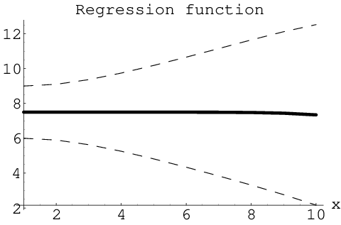


Acknowledgements The author wants to thank Federico Girosi, Tomaso Poggio, Jörg Uhlig, and Achim Weiguny for discussions.
References
- [1] Aarts, E. & Korts, J. (1989) Simulated Annealing and Boltzmann Machines. New York: Wiley.
- [2] Abu–Mostafa, Y. (1990) Learning from Hints in Neural Networks. Journal of Complexity 6, 192–198.
- [3] Abu–Mostafa, Y. (1993) Hints and the VC Dimension. Neural Computation 5, 278–288.
- [4] Abu–Mostafa, Y. (1993b) A method for learning from hints. Advances in Neural Information Processing Systems 5, S. Hanson et al (eds.), 73–80, San Mateo, CA: Morgan Kauffmann.
- [5] Aida, T. (1999) Field Theoretical Analysis of On-line Learning of Probability Distributions. Phys. Rev. Lett. 83, 3554-3557, arXiv:cond-mat/9911474.
- [6] Allen, D.M. (1974) The relationship between variable selection and data augmentation and a method of prediction. Technometrics 16, 125.
- [7] Amari, S., Cichocki, A., & Yang, H.H.(1996) A New Learning Algorithm for Blind Signal Separation. in Advances in Neural Information Processing Systems 8, D.S. Touretzky et al (eds.), 757–763, Cambridge, MA: MIT Press.
- [8] Ames, W.F. (1977) Numerical Methods for Partial Differential Equations. (2nd. ed.) New York: Academic Press.
- [9] Balian, R. (1991) From Microphysics to Macrophysics. Vol. I. Berlin: Springer Verlag.
- [10] Ballard, D.H. (1997) An Introduction to Natural Computation. Cambridge, MA: MIT Press.
- [11] Bazaraa, M.S., Sherali, H.D., & Shetty, C.M. (1993) Nonlinear Programming. (2nd ed.) New York: Wiley.
- [12] Bayes, T.R. (1763) An Essay Towards Solving a Problem in the Doctrine of Chances. Phil. Trans. Roy. Soc. London 53, 370. (Reprinted in Biometrika (1958) 45, 293)
- [13] Beck, C. & Schlögl, F. (1993) Thermodynamics of chaotic systems. Cambridge: Cambridge University Press.
- [14] Bell, A.J. & Sejnowski, T.J. (1995) Neural Computation 7(6), 1129–1159.
- [15] Ben–Israel, A. & Greville, Th.N.E. (1974) Generalized Inverses. New York: Wiley.
- [16] Berger, J.O. (1980) Statistical Decision Theory and Bayesian Analysis. New York: Springer Verlag.
- [17] Berger, J.O. & Wolpert R. (1988) The Likelihood Principle. (2nd ed.) Hayward, CA: IMS Lecture Notes — Monograph Series 9.
- [18] Bernado, J.M. & Smith, A.F. (1994) Bayesian Theory. New York: John Wiley.
- [19] Bertsekas, D.P. (1995) Nonlinear Programming. Belmont, MA: Athena Scientific.
- [20] Bialek, W., Callan, C.G., & Strong, S.P. (1996) Field Theories for Learning Probability Distributions. Phys. Rev. Lett. 77, 4693-4697, arXiv:cond-mat/9607180.
- [21] Binder, K. & Heermann, D.W. (1988) Monte Carlo simulation in statistical physics: an introduction. Berlin: Springer Verlag.
- [22] Bishop, C.M. (1993) Curvature–driven smoothing: a learning algorithm for feedforward netsworks. IEEE Transactions on Neural Networks 4(5),882–884.
- [23] Bishop, C.M. (1995) Training with noise is equivalent to Tikhonov regularization. Neural Computation 7 (1), 108–116.
- [24] Bishop, C.M. (1995) Neural Networks for Pattern Recognition. Oxford: Oxford University Press.
- [25] Bishop, E. & Bridges, D. (1985) Constructive Analysis. Grundlehren der Mathematischen Wissenschaften, Vol. 279. Berlin: Springer Verlag.
- [26] Black, M.J. & Rangarajan, A. (1996) On the Unification of Line Processes, Outlier Rejection, and Robust Statistics With Applications in Early Vision. Int’l J. Computer Vision 19 (1).
- [27] Blaizot, J.–P. & Ripka, G. (1986) Quantum Theory of Finite Systems. Cambridge, MA: MIT Press.
- [28] Blake, A. & Zisserman, A. (1987) Visual reconstruction Cambridge, MA: MIT Press.
- [29] Blanchard, P. & Bruening, E. (1982) Variational Methods in Mathematical Physics. Berlin: Springer Verlag.
- [30] Bleistein, N. & Handelsman, N. (1986) Asymptotic Expansions of Integrals. (Originally published in 1975 by Holt, Rinehart and Winston, New York) New York: Dover.
- [31] Breiman, L. (1993) Hinging hyperplanes for regression, classification, and function approximation. IEEE Trans. Inform. Theory 39(3), 999–1013.
- [32] Breiman, L., Friedman, J.H., Olshen, R.A., & Stone, C.J. (1993) Classification and Regression Trees, New York: Chapman & Hall.
- [33]
Bretthorst, G.L. (1988)
Bayesian spectrum analysis and parameter estimation.
Lecture Notes in Statistics, Vol. 48.
Berlin: Springer Verlag.
(Available at http://bayes.wustl.edu/glb/book.pdf) - [34] Cardy, J. (1996) Scaling and Renormalization in Statistical Physics. Cambridge: Cambridge University Press.
- [35] Carlin, B.P. & T.A. Louis (1996) Bayes and Empirical Bayes Methods for Data Analysis. Boca Raton: Chapman & Hall/CRC.
- [36] Choquet–Bruhat Y., DeWitt–Morette, C., & Dillard–Bleick, M. (1982) Analysis, Manifolds, and Physics. Part I. Amsterdam: North–Holland.
- [37] Collins, J. (1984) Renormalization. Cambridge: Cambridge University Press.
- [38] Cox, D.R. & Hinkley, D.V. (1974) Theoretical Statistics. London: Chapman & Hall.
- [39] Craven, P. & Wahba, G. (1979) Smoothing noisy data with spline functions: estimating the correct degree of smoothing by the method of generalized cross–validation. Numer.Math. 31, 377–403.
- [40] Cressie, N.A.C. (1993) Statistics for Spatial Data. New York, Wiley.
- [41] Creutz, M. (1983) Quarks, gluons and lattices. Cambridge: Cambridge University Press.
- [42] D’Agostini, G. (1999) Bayesian Reasoning in High Energy Physics. — Principles and Applications — CERN Yellow Report 99–03 (Available at http://www-zeus.roma1.infn.it/∼agostini/prob+stat.html)
- [43] Davis, L. (ed.) (1987) Genetic Algorithms and Simulated Annealing. San Mateo, CA: Morgan Kaufmann.
- [44] Davis, L. (ed.) (1991) Handbook of Genetic Algorithms New York: Van Nostrand Reinhold.
- [45] De Bruijn, N.G. (1981) Asymptotic Methods in Analysis. (Originally published in 1958 by the North–Holland Publishing Co., Amsterdam) New York: Dover.
- [46] Deco, G. & Obradovic, D. (1996) An Information–Theoretic Approach to Neural Computing. New York: Springer Verlag.
- [47] Devroye, L., Györfi, L., & Lugosi, G. (1996) A Probabilistic Theory of Pattern recognition. New York: Springer Verlag.
- [48] Di Castro, C. & Jona-Lasinio, G. (1976) The Renormalization Group Approach to Critical Phenomena. In: Domb, C. & Green M.S. (eds.) Phase Transitions and Critical Phenomena. London: Academic Press.
- [49] Dietrich, R., Opper, M., & Sompolinsky, H. (1999) Statistical Mechanics of Support Vector Networks. Physical Review Letters 82(14), 2975–2978.
- [50] Donoho, D.L. & Johnstone, I.M. (1989) Projection–based approximation and a duality with kernel methods. Ann.Statist. 17(1),58–106.
- [51] Doob, J.L. (1953) Stochastic Processes. (New edition 1990) New York: Wiley.
- [52] Dudley, R.M. (1984) A course on empirical processes. Lecture Notes in Mathematics 1097,2-142.
- [53] Ebeling, W., Freund, J., & Schweitzer, F. (1998) Komplexe Strukturen: Entropie und Information. Stuttgart: Teubner.
- [54] Efron, B. & Tibshirani R.J. (1993) An Introduction to the Bootstrap. New York: Chapman & Hall.
- [55] Eisenberg, J. & Greiner, W. (1972) Microscopic Theory of the Nucleus. North–Holland, Amsterdam.
- [56] Fernández, R., Fröhlich, J., & Sokal, A.D. (1992) Random Walks, Critical Phenomena, and Triviality in Quantum Field Theory. Berlin: Springer Verlag.
- [57] Fletcher, R. (1987) Practical Methods of Optimization. New York: Wiley.
- [58] Fredholm I. (1903) Acta Math. 27.
- [59] Friedman, J.H. & Tukey, J.W. (1974) A projection pursuit algorithm for exploratory data analysis. IEEE Trans. Comput. 24, 1000–1006.
- [60] Friedman, J.H. & Stuetzle, W. (1981) Projection pursuit regression. J.Am.Statist.Assoc. 76(376), 817–823.
- [61] Fukunaga, K. (1990) Statistical Pattern Recognition Boston: Academic Press.
- [62] Gardner, E. (1987) Maximum Storage Capacity in Neural Networks. Europhysics Letters 4 481–485.
- [63] Gardner, E. (1988) The Space of Interactions in Neural Network Models. Journal of Physics A 21 257–270.
- [64] Gardner, E. & Derrida B. (1988) Optimal Storage Properties of Neural Network Models. Journal of Physics A 21 271–284.
- [65] Gardiner, C.W. (1990) Handbook of Stochastic Methods. (2nd ed.) Berlin: Springer Verlag.
- [66] Geiger, D. & Girosi, F. (1991) Parallel and Deterministic Algortihms for MRFs: Surface Reconstruction. IEEE Trans. on Pattern Analysis and Machine Intelligence 13 (5), 401–412.
- [67] Geiger, D. & Yuille, A.L. (1991) A Common Framework for Image Segmentation. Int’l J. Computer Vision 6 (3), 227–243.
- [68] Gelfand, S.B. & Mitter, S.K. (1993) On Sampling Methods and Annealing Algorithms. Markov Random Fields – Theory and Applications. New York: Academic Press.
- [69] Gelman, A., Carlin, J.B., Stern, H.S., & Rubin, D.B. (1995) Bayesian Data Analysis. New York: Chapman & Hall.
- [70] Geman, S. & Geman, D. (1984) Stochastic relaxation, Gibbs distributions and the Bayesian restoration of images. IEEE Trans. on Pattern Analysis and Machine Intelligence 6, 721–741. Reprinted in Shafer & Pearl (eds.) (1990) Readings in Uncertainty Reasoning. San Mateo, CA: Morgan Kaufmann.
- [71] Geman, D. & Reynoids, G. (1992) Constraint restoration and the Recover of Discontinuities. IEEE Trans. on Pattern Analysis and Machine Intelligence. 14, 367–383.
- [72] Giraud, B.G., Lapedes, A., Liu, L.C., & Lemm, J.C. (1995) Lorentzian Neural Nets. Neural Networks 8 (5), 757-767.
- [73] Girosi, F. (1991) Models of noise and robust estimates. A.I.Memo 1287, Artificial Intelligence Laboratory, Massachusetts Institute of Technology.
- [74] Girosi, F., (1997) An equivalence between sparse approximation and support vector machines. A.I. Memo No.1606, Artificial Intelligence Laboratory, Massachusetts Institute of Technology.
- [75] Girosi, F., Poggio, T., & Caprile, B. (1991) Extensions of a theory of networks for approximations and learning: Outliers and negative examples. In Lippmann, R., Moody, J., & Touretzky, D. (eds.) Advances in Neural Information Processing Systems 3, San Mateo, CA: Morgan Kaufmann.
- [76] Girosi, F., Jones, M., & Poggio, T. (1995) Regularization Theory and Neural Networks Architectures. Neural Computation 7 (2), 219–269.
- [77] Glimm, J. & Jaffe, A. (1987) Quantum Physics. A Functional Integral Point of View. New York: Springer Verlag.
- [78] Goeke, K., Cusson, R.Y., Gruemmer, F., Reinhard, P.–G., Reinhardt, H., (1983) Prog. Theor. Physics [Suppl.] 74 & 75, 33.
- [79] Goldberg, D.E. (1989) Genetic Algorithms in Search, Optimization, and Machine Learning. Redwood City, CA: Addison–Wesley.
- [80] Golden, R.M. (1996) Mathematical Methods for Neural Network Analysis and Design. Cambridge, MA: MIT Press.
- [81] Golup, G., Heath, M., & Wahba, G.(1979) Generalized cross validation as a method for choosing a good ridge parameter. Technometrics 21, 215–224.
- [82] Good, I.J. & Gaskins, R.A. (1971) Nonparametric roughness penalties for probability densities. Biometrika 58, 255–277.
- [83] Green, P.J. & Silverman, B.W. (1994) Nonparametric Regression and Generalized Linear Models. London: Chapman & Hall.
- [84] Großman, Ch. & Roos H.–G. (1994) Numerik partieller Differentialgleichungen. Stuttgart: Teubner.
- [85] Gull, S.F. (1988) Bayesian data analysis – straight line fitting. In Skilling, J, (ed.) Maximum Entropy and Bayesian Methods. Cambridge, 511 –518, Dordrecht: Kluwer.
- [86] Gull, S.F. (1989) Developments in maximum entropy data analysis. In Skilling, J, (ed.) Maximum Entropy and Bayesian Methods. Cambridge 1988, 53 – 71, Dordrecht: Kluwer.
- [87] Hackbusch, W. (1985) Multi–grid Methods and Applications. New York: Springer Verlag.
- [88] Hackbusch, W. (1989) Integralgleichungen. Teubner Studienbücher. Stuttgart: Teubner.
- [89] Hackbusch, W. (1993) Iterative Lösung großer schwachbesetzter Gleichungssysteme. Teubner Studienbücher. Stuttgart: Teubner.
- [90] Härdle, W. (1990) Applied nonparametric regression. Cambridge: Cambridge University Press.
- [91] Hammersley, J.M. & Handscomb, D.C. (1964) Monte Carlo Methods. London: Chapman & Hall.
- [92] Hastie, T.J. & Tibshirani, R.J. (1986) Generalized Additive Models. Statist.Sci. 1,297–318.
- [93] Hastie, T.J. & Tibshirani, R.J. (1987) Generalized Additive Models: Some applications. J.Am.Statist.Assoc. 82,371–386.
- [94] Hastie, T.J. & Tibshirani, R.J. (1990) Generalized Additive Models. London: Chapman & Hall.
- [95] Hastings, W.K. (1970) Monte Carlo sampling methods using Markov chains and their applications. Biometrika 57, 97–109.
- [96] Hertz, J., Krogh, A. & Palmer, R.G. (1991) Introduction to the Theory of Neural Computation. Santa Fe Institute, Lecture Notes Volume I, Addison–Wesley.
- [97] Hilbert, D. & Courant,R. (1989) Methods of Mathematical Physics Vol.1&2,(1st German editions 1924,1937, Springer Verlag) New York: Wiley.
- [98] Holland, J.H. (1975) Adaption in Natural and Artificial Systems. University of Michigan Press. (2nd ed. MIT Press, 1992.)
- [99] Horst, R., Pardalos, M., & Thoai, N.V. (1995) Introduction to Global Optimization. Dordrecht: Kluwer.
- [100] Huber, P.J. (1979) Robust Smoothing. In Launer, E. & Wilkinson G. (eds.) Robustness in Statistics New York: Academic Press.
- [101] Huber, P.J. (1981) Robust Statistics. New York: Wiley.
- [102] Huber, P.J. (1985) Projection Pursuit. Ann.Statist. 13(2),435–475.
- [103] Itzkyson, C. & Drouffe, J.–M. (1989) Statistical Field Theory. (Vols. 1 and 2) Cambridge: Cambridge University Press.
- [104] Jaynes, E.T. (in preparation) Probability Theory: The Logic Of Science. (Available at http://bayes.wustl.edu/etj/prob.html)
- [105]
Jeffrey, R. (1999).
Probabilistic Thinking.
(Available at http://www.princeton.edu/∼bayesway/) - [106] Jeggle, H. (1979) Nichtlineare Funktionalanalysis. Stuttgart: Teubner.
- [107] Jensen, F.V. (1996) An Introduction to Bayesian Networks. New York: Springer Verlag.
- [108] Jones, M.C. & Sibson, R. (1987) What is Projection Pursuit? J. Roy. Statist. Soc. A 150, 1–36.
- [109] Kaku, M. (1993) Quantum Field Theory. Oxford: Oxford University Press.
- [110] van Kampen, N.G. (1992) Stochastic Processes in Physics and Chemistry. Amsterdam: North–Holland.
- [111] Kant, I. (1911) Kritik der reinen Vernunft.(2nd ed.) Werke, Vol.3 Berlin: Königliche Akademie der Wissenschaften.
- [112] Kimmeldorf, G.S. & Wahba, G. (1970) A correspondence between Bayesian estimation on stochastic processes and smoothing splines. Ann. Math. Stat. 41, 495–502.
- [113] Kimmeldorf, G.S. & Wahba, G. (1970) Spline functions and stochastic processes. Sankhya Ser. A 32, Part 2, 173–180.
- [114] Kirkpatrick, S., Gelatt Jr., C.D., & Vecchi, M.P. (1983) Optimization by Simulated Annealing. Science 220, 671–680.
- [115] Kirsch, A. (1996) An Introduction to the Mathematical Theory of Inverse Problems. New York: Springer Verlag.
- [116] Kitagawa, G., Gersch, W. (1996) Smoothness Priors Analysis of Time Series New York: Springer Verlag.
- [117] Kleinert, H.(1993) Pfadintegrale. Mannheim: Wissenschaftsverlag.
- [118] Klir, G.J. & Yuan, B. (1995) Fuzzy Sets and Fuzzy Logic. Prentice Hall.
- [119] Klir, G.J. & Yuan, B. (eds.) (1996) Fuzzy Sets, Fuzzy Logic, and Fuzzy Systems. World Scientific.
- [120] Koecher, M. (1985) Lineare Algebra und analytische Geometrie. Berlin: Springer Verlag.
- [121] Koza, J.R. (1992) Genetic Programming Cambridge, MA: MIT Press.
- [122] Kullback, S. & Leibler R.A. (1951) On Information and Sufficiency. Ann.Math.Statist. 22, 79–86.
- [123] Kullback, S. (1951) Information Theory and Statistics. New York: Wiley.
- [124] Lapedes, A. & Farber, R. (1988) How neural nets work. in Neural Information Processing Systems, D.Z.Anderson, (ed.),442–456. New York: American Institute of Physics.
- [125] Lauritzen, S.L. (1996) Graphical Models. Oxford: Clarendon Press.
- [126] Le Bellac, M. (1991) Quantum and Statistical Field Theory. Oxford Science Publications, Oxford: Clarendon Press.
- [127] Le Cam, L. (1986) Asymptotic Methods in Statistical Decision Theory. New York: Springer Verlag.
- [128] Leen, T.K. (1995) From Data Distributions to Regularization in Invariant Learning. Neural Computation 7, 974–981.
- [129] Lemm, J.C. (1995) Inhomogeneous Random Phase Approximation for Nuclear and Atomic Reactions. Annals of Physics 244 (1), 136–200, 1995.
- [130] Lemm, J.C. (1995) Inhomogeneous Random Phase Approximation: A Solvable Model. Annals of Physics 244 (1), 201–238, 1995.
- [131] Lemm, J.C. (1996) Prior Information and Generalized Questions. A.I.Memo No. 1598, C.B.C.L. Paper No. 141, Massachusetts Institute of Technology. (Available at http://pauli.uni-muenster.de/∼lemm)
- [132] Lemm, J.C. (1998) How to Implement A Priori Information: A Statistical Mechanics Approach. Technical Report MS-TP1-98-12, Münster University, arXiv:cond-mat/9808039.
- [133] Lemm, J.C. (1998) Fuzzy Interface with Prior Concepts and Non-Convex Regularization. In Wilfried Brauer (Ed.), Proceedings of the 5. International Workshop ”Fuzzy-Neuro Systems ’98” (FNS ’98), March 19-20, 1998, Munich, Germany, Sankt Augustin: Infix.
- [134] Lemm, J.C. (1998) Quadratic Concepts. In Niklasson L., Bodén, M., & Ziemke, T. (eds.) Proceedings of the 8th International Conference on Artificial Neural Networks. (ICANN98) New York: Springer Verlag.
- [135] Lemm, J.C. (1998) Fuzzy Rules and Regularization Theory. In ELITE European Laboratory for Intelligent Techniques Engineering (ed.): Proceedings of the 6th European Congress on Intelligent Techniques and Soft Computing (EUFIT ’98), Aachen, Germany, September 7-10, 1998, Mainz, Aachen.
- [136] Lemm, J.C. (1999) Mixtures of Gaussian Process Priors. In Proceedings of the Ninth International Conference on Artificial Neural Networks (ICANN99), IEEE Conference Publication No. 470. London: Institution of Electrical Engineers.
- [137] Lemm, J.C. (2000) Inverse Time–dependent Quantum Mechanics. Technical Report, MS-TP1-00-1, Münster University, arXiv:quant-ph/0002010.
- [138] Lemm, J.C., Beiu, V., & Taylor, J.G. (1995) Density Estimation as a Preprocessing Step for Constructive Algorithms. In Kappen B., Gielen, S. (eds.): Proceedings of the 3rd SNN Neural Network Symposium. The Netherlands, Nijmegen, 14–15 September 1995, Berlin, Springer Verlag.
- [139] Lemm, J.C., Giraud, B.G., & Weiguny, A. (1990) Mean field approximation versus exact treatment of collisions in few–body systems. Z.Phys.A – Atomic Nuclei 336, 179–188.
- [140] Lemm, J.C., Giraud, B.G., & Weiguny, A. (1994) Beyond the time independent mean field theory for nuclear and atomic reactions: Inclusion of particle-hole correlations in a generalized random phase approximation. Phys.Rev.Lett. 73, 420, arXiv:nucl-th/9911056.
- [141] Lemm, J.C. & Uhlig, J. (1999) Hartree-Fock Approximation for Inverse Many-Body Problems. Technical Report, MS-TP1-99-10, Münster University, arXiv:nucl-th/9908056.
- [142] Lemm, J.C., Uhlig J., & Weiguny, A. (2000) Bayesian Approach to Inverse Quantum Statistics. Phys. Rev. Lett. 84, 2068. arXiv:cond-mat/9907013.
- [143] Lifshits, M.A. (1995) Gaussian Random Functions. Dordrecht: Kluwer.
- [144]
Loredo T. (1990)
From Laplace to Supernova SN 1987A: Bayesian Inference in Astrophysics.
In Fougère, P.F. (ed.)
Maximum-Entropy and Bayesian Methods, Dartmouth, 1989, 81–142.
Dordrecht: Kluwer.
(Available at http://bayes.wustl.edu/gregory/gregory.html) - [145] Louis, A.K. (1989) Inverse und schlecht gestellte Probleme. Stuttgart: Teubner.
- [146] MacKay, D.J.C. (1992) The evidence framework applied to classification networks. Neural Computation 4 (5), 720–736.
- [147] MacKay, D.J.C. (1992) A practical Bayesian framework for backpropagation networks. Neural Computation 4 (3), 448–472.
- [148] MacKay, D.J.C. (1994) Hyperparameters: optimise or integrate out? In Heidbreder, G. (ed.) Maximum Entropy and Bayesian Methods, Santa Barbara 1993. Dordrecht: Kluwer.
- [149] MacKay, D.J.C. (1998) Introduction to Gaussian processes. In Bishop, C., (ed.) Neural Networks and Machine Learning. NATO Asi Series. Series F, Computer and Systems Sciences, Vol. 168.
- [150] Marroquin, J.L., Mitter, S., & Poggio, T. (1987) Probabilistic solution of ill–posed problems in computational vision. J. Am. Stat. Assoc. 82, 76–89.
- [151] Metropolis, N., Rosenbluth, A.W., Rosenbluth, M.N., Teller, A.H., & Teller, E. (1953) Equation of state calculations by fast computing machines. Journal of Chemical Physics 21, 1087–1092.
- [152] McCullagh, P. & Nelder, J.A. (1989) Generalized Linear Models London: Chapman & Hall.
- [153] Mezard, M., Parisi, G., & Virasoro, M.A. (1987) Spin Glass Theory and Beyond. Singapore: World Scientific.
- [154] Michalewicz, Z. (1992) Genetic Algorithms + Data Structures = Evolution Programs. Berlin: Springer Verlag.
- [155] Michie, D., Spiegelhalter, D.J., & Taylor, C.C. (Eds.) (1994) Machine Learning, Neural and Statistical Classification. New York: Ellis Horwood.
- [156] Minski, M.L. & Papert, S.A. (1990) Perceptrons. (Expanded Edition, Original edition, 1969) Cambridge, MA: MIT Press.
- [157] Mitchell, M. (1996) An Introduction to Genetic Algorithms. Cambridge, MA: MIT Press.
- [158] Mitchell, A.R. & Griffiths, D.F. (1980) The Finite Difference Method in Partial Differential Equations. New York: Wiley.
- [159] Molgedey, L. & Schuster, H.G. (1994) Separation of a mixture of independent signals using time delayed correlations. Phys.Rev.Lett. 72(23), 3634–3637.
- [160] Montvay, I. & Münster, G. (1994) Quantum Fields on a Lattice. Cambridge: Cambridge University Press.
- [161] Moore, E.H. (1920) Bull.Amer.Math.Soc. 26.
- [162] Morozov, V.A. (1984) Methods for Solving Incorrectly Posed problems. New York: Springer Verlag.
- [163] Mosteller, F. & Wallace, D. (1963) Inference in an authorship problem. A comparative study of discrimination methods applied to authorships of the disputed Federalist papers. J. Amer. Statist. Assoc. 58, 275–309.
- [164] Müller, B. & Reinhardt, J. (1991) Neural Networks. (2nd printing) Berlin, Springer Verlag.
- [165] Mumford, D. & Shah, J. (1989) Optimal Approximations by Piecewise Smooth Functions and Associated Variational Problems. Comm. Pure Applied Math. 42, 577–684.
- [166] Nadaraya, E.A. (1965) On nonparametric estimates of density functions and regression curves. Theor.Prob.Appl. 10,186–190.
- [167] Neal, R.M. (1996) Bayesian Learning for Neural Networks. New York: Springer Verlag.
- [168] Neal, R.M. (1997) Monte Carlo Implementation of Gaussian Process Models for Bayesian Regression and Classification. Technical Report No. 9702, Dept. of Statistics, Univ. of Toronto, Canada.
- [169] Negele, J.W. & Orland, H. (1988) Quantum Many–Particle Systems. Frontiers In Physics Series (Vol. 68), Redwood City, CA: Addison–Wesley.
- [170] Nitzberg, M. & Shiota T. (1992) Nonlinear Image Filtering With Edge and Corner Enhancement. IEEE Trans. on Pattern Analysis and Machine Intelligence. 14, (8) 862-833.
- [171] O’Hagen, A. (1994) Kendall’s advanced theory of statistics, Vol. 2B: Bayesian inference. London: Edward Arnold.
- [172] Olshausen, B.A. & Field, D.J. (1995) Natural Image Statistics and Efficient Coding. Workshop on Information Theory and the Brain, Sept. 4–5, 1995, University of Stirling. Proceedings published in Network 7, 333-339.
- [173] Olshausen, B.A. & Field, D.J. (1996) Emergence of simple–cell receptive field properties by learning a spares code for natural images. Nature 381, 607–609.
- [174] Opper, M. (1999) Gaussian Processes for Classification: Mean Field Algorithms. Tech Report NCRG/1999/030, Neural Computing Research Group at Aston University, UK.
- [175] Opper, M. & Kinzel, W. (1996) Statistical Mechanics of Generalization. In Domany, E., van Hemmen, J.L., & Schulten, K. (eds.) Models of Neural Networks III. New York: Springer Verlag.
- [176] Opper, M., & Winther, O. (1999) Mean field methods for classification with Gaussian processes. In Kearns, M.S., Solla, S.S., & Cohn D.A. (eds.) Advances in Neural Information Processing Systems 11, 309–315, Cambridge, MA: MIT Press.
- [177] Ó Ruanaidh, J.J.K. & Fitzgerald W.J. (1996) Numerical Bayesian Methods Applied to Signal Processing. New York: Springer Verlag.
- [178]
Parzen, E. (1962)
An approach to time series analysis.
Ann.Math.Statist. 32, 951–989. - [179] Parzen, E. (1962) On the estimation of a probability function and mode. Ann.Math.Statist. 33(3).
- [180] Parzen, E. (1963) Probability density functionals and reproducing kernel Hilbert spaces. In Rosenblatt, M.(ed.) Proc. Symposium on Time Series Analysis, 155–169, New York: Wiley.
- [181] Parzen, E. (1970) Statistical inference on time series by rkhs methods. In Pyke, R.(ed.) Proc. 12th Biennal Seminar, 1–37, Montreal, Canada: Canadian Mathematical Congress.
- [182] Pearl, J. (1988) Probabilistic Reasoning in Intelligent Systems. San Mateo, CA: Morgan Kauffmann.
- [183] Perona, P. & Malik J. (1990) Scale–Space and Edge Detection Using Anisotropic Diffusion. IEEE Trans. on Pattern Analysis and Machine Intelligence. 12(7), 629–639.
- [184] Perskin, M.E. & Schroeder, D.V. (1995) An Introduction to Quantum Field Theory. Reading, MA, Addison–Wesley.
- [185] Pierre, D.A. (1986) Optimization Theory with Applications. New York: Dover. (Original edition Wiley, 1969).
- [186] Poggio, T. & Girosi, F. (1990) Networks for Approximation and Learning. Proceedings of the IEEE, Vol 78, No. 9.
- [187] Poggio, T., Torre, V., & Koch, C. (1985) Computational vision and regularization theory. Nature 317, 314–319.
- [188] Polak, E. (1997) Optimization. New York: Springer Verlag.
- [189] Pollard, D. (1984) Convergence of Stochastic Processes. New York: Springer Verlag.
- [190] Pordt, A. (1998) Random Walks in Field Theory In Meyer–Ortmanns, H, Klümper A. (eds.) (1998) Field Theoretical Tools for Polymer and Particle Physics. Berlin: Springer Verlag.
- [191] Press, W.H., Teukolsky, S.A., Vetterling, W.T., & Flannery, B.P. (1992) Numerical Recipes in C. Cambridge: Cambridge University Press.
- [192] Ryder, L.H. (1996) Quantum Field Theory. Cambridge: Cambridge University Press.
- [193] Ring, P., & Schuck, P. (1980) The Nuclear Many–Body Problem. New York: Springer Verlag.
- [194] Ripley, B.D. (1977) Modelling spatial patterns (with discussion). Journal of the Royal Statistical Society series B 39, 172–212.
- [195] Ripley, B.D. (1987) Stochastic Simulation. New York: Wiley.
- [196] Ripley, B.D. (1996) Pattern Recognition and Neural Networks. Cambridge: Cambridge University Press.
- [197] Robert, C.P. (1994) The Bayesian Choice. New York: Springer Verlag.
- [198] Rodriguez, C.C. (1997) Cross validated Non Parametric Bayesianism by Markov Chain Monte Carlo. arXiv:nucl-th/9908056.
- [199] Rose, K., Gurewitz, E., & Fox, G.C. (1990) Statistical mechanics and phase transitions in clustering. Phys. Rev. Lett. 65, 945–948.
- [200] Rothe, H.J. (1992) Lattice Gauge Theories. Singapore: World Scientific.
- [201] Rumelhart, D.E., McClelland, J.L., and the PDP Research Group (1986) Parallel Distributed Processing, vol.1& 2, Cambridge, MA: MIT Press.
- [202] Schervish, M.J. (1995) Theory of Statistics. New York: Springer Verlag.
- [203] Schölkopf, B., Burges C., & Smola, A. (1998) Advances in Kernel Methods: Support Vector Machines. Cambridge, MA: MIT Press.
- [204] Schwefel, H.–P. (1995) Evolution and Optimum Seeking. New York: Wiley.
- [205] Silverman, B.W. (1984) Spline smoothing: The equivalent variable kernel method. Ann. Statist. 12, 898–916. London: Chapman & Hall.
- [206] Silverman, B.W. (1986) Density Estimation for Statistics and Data Analysis. London: Chapman & Hall.
- [207] Sivia, D.S. (1996) Data Analysis: A Bayesian Tutorial. Oxford: Oxford University Press.
- [208] Skilling, J. (1991) On parameter estimation and quantified MaxEnt. In Grandy, W.T. & Schick, L.H. (eds.) Maximum Entropy and Bayesian Methods. Laramie, 1990, 267 –273, Dordrecht: Kluwer.
- [209] Smola A.J. & Schölkopf, B, (1998) From regularization operators to support vector kernels. In: Jordan, M.I., Kearns, M.J., & Solla S.A. (Eds.): Advances in Neural Information Processing Systems 10. Cambridge, MA: MIT Press.
- [210] Smola A.J., Schölkopf, B, & Müller, K–R. (1998) The connection between regularization operators and support vector kernels. Neural Networks 11, 637–649.
- [211] Stone, M. (1974) Cross–validation choice and assessment of statistical predictions. Journal of the Royal Statistical Society B 36, 111-147.
- [212] Stone, M. (1977) An asymptotic equivalence of choice of model by cross–validation and Akaike’s criterion. Journal of the Royal Statistical Society B 39, 44.
- [213] Stone, C.J. (1985) Additive regression and other nonparametric models. Ann.Statist. 13,689–705.
- [214] Tierney, L. (1994) Markov chains for exploring posterior distributions (with discussion). Annals of Statistics 22, 1701–1762.
- [215] Tikhonov, A.N. (1963) Solution of incorrectly formulated problems and the regularization method. Soviet Math. Dokl. 4, 1035–1038.
- [216] Tikhonov, A.N. & Arsenin, V.Y. (1977) Solution of Ill–posed Problems. Washington, DC: W.H.Winston.
- [217] Uhlig, J. (In preparation) PhD Thesis, Münster University.
- [218] Uhlig, J., Lemm, J., & Weiguny, A. (1998) Mean field methods for atomic and nuclear reactions: The link between time–dependent and time–independent approaches. Eur. Phys. A 2, 343–354.
- [219] Vapnik, V.N. (1982) Estimation of dependencies based on empirical data. New York: Springer Verlag.
- [220] Vapnik, V.N. (1995) The Nature of Statistical Learning Theory. New York: Springer Verlag.
- [221] Vapnik, V.N. (1998) Statistical Learning Theory. New York: Wiley.
- [222] Vico, G. (1858, original 1710) De antiquissima Italorum sapientia Naples: Stamperia de’ Classici Latini.
- [223] Wahba, G. (1990) Spline Models for Observational Data. Philadelphia: SIAM.
- [224] Wahba, G. (1997) Support vector machines, reproducing kernel Hilbert spaces and the randomized GACV. Technical Report 984, University of Wisconsin.
- [225] Wahba, G. & Wold, S. 1975) A completely automatic French curve. Commun. Statist. 4, 1–17.
- [226] Watkin, T.L.H., Rau, A., & Biehl, M. (1993) The statistical mechanics of learning a rule. Rev. Mod. Phys. 65, 499–556.
- [227] Watzlawick, P. (ed.) (1984) The Invented Reality. New York: Norton.
- [228] Weinstein, S. (1995) The Quantum Theory of Fields. Vol.1 Cambridge: Cambridge University Press.
- [229] Weinstein, S. (1996) The Quantum Theory of Fields. Vol.2 Cambridge: Cambridge University Press.
- [230] West, M & Harrison, J. (1997) Bayesian Forecasting and Dynamic Models. New York, Springer Verlag.
- [231] Williams, C.K.I. & Barber, D. (1998) Bayesian Classification With Gaussian Processes IEEE Trans. on Pattern Analysis and Machine Intelligence. 20(12), 1342–1351.
- [232] Williams, C.K.I. & Rasmussen, C.E. (1996) Gaussian Processes for Regression. in Advances in Neural Information Processing Systems 8, D.S. Touretzky et al (eds.), 515–520, Cambridge, MA: MIT Press.
- [233] Winkler, G. (1995) Image Analysis, Random Fields and Dynamic Monte Carlo Methods. Berlin: Springer Verlag.
- [234] Wolpert, D.H. (ed.) (1995) The Mathematics of Generalization. The Proceedings of the SFI/CNLS Workshop on Formal Approaches to Supervised Learning. Santa Fe Institute, Studies in the Sciences of Complexity. Reading, MA: Addison–Wesley.
- [235] Wolpert, D.H. (1996) The Lack of A Priori Distinctions between Learning Algorithms. Neural Computation 8 (7), 1341-1390.
- [236] Wolpert, D.H. (1996) The Existence of A Priori Distinctions between Learning Algorithms. Neural Computation 8 (7), 1391-1420.
- [237] Yakowitz, S.J. & Szidarovsky, F. (1985) A Comparison of Kriging With Nonparametric Regression Methods. J.Multivariate Analysis. 16, 21-53.
- [238] Yuille, A.L., (1990) Generalized deformable models, statistical physics and matching problems. Neural Computation, 2, (1) 1–24.
- [239] Yuille, A.L. & Kosowski, J.J. (1994) Statistical Physics Algorithm That Converge. Neural Computation 6 (3), 341–356.
- [240] Yuille, A.L., Stolorz, P., & Utans, J. (1994) Statistical Physics, Mixtures of Distributions, and EM Algorithm. Neural Computation, 6 (2), 334–340.
- [241] Zhu, S.C. & Yuille, A.L. (1996) Region Competition: Unifying Snakes, Region Growing, and Bayes/MDL for Multiband Image Segmentation. IEEE Trans. on Pattern Analysis and Machine Intelligence 18 (9), 884–900.
- [242] Zhu, S.C. & Mumford, D.´ (1997) Prior Learning and Gibbs Reaction–Diffusion. IEEE Trans. on Pattern Analysis and Machine Intelligence 19 (11), 1236–1250.
- [243] Zhu, S.C., Wu, Y.N., & Mumford, D. (1997) Minimax Entropy principle and Its Application to Texture Modeling. Neural Computation, 9 (8).
- [244] Zinn–Justin, J. (1989) Quantum Field Theory and Critical Phenomena. Oxford: Oxford Science Publications.