Kulback-Leibler and Renormalized Entropy: Applications to EEGs of Epilepsy Patients

R. Quian Quiroga Affiliation: John von Neumann Institute for Computing,Forschungszentrum Jülich GmbH,D - 52425 Jülich, Germany J. Arnhold K. Lehnertz Affiliation: Clinic of Epileptology, University of Bonn,Sigmund-Freud Str. 25,D - 53105 Bonn, Germany and P. Grassberger Affiliation: John von Neumann Institute for Computing,Forschungszentrum Jülich GmbH,D - 52425 Jülich, Germany

Recently, “renormalized entropy” was proposed as a novel measure of relative entropy (P. Saparin et al., Chaos, Solitons & Fractals 4, 1907 (1994)) and applied to several physiological time sequences, including EEGs of patients with epilepsy. We show here that this measure is just a modified Kullback-Leibler (K-L) relative entropy, and it gives similar numerical results to the standard K-L entropy. The latter better distinguishes frequency contents of e.g. seizure and background EEGs than renormalized entropy. We thus propose that renormalized entropy might not be as useful as claimed by its proponents. In passing we also make some critical remarks about the implementation of these methods.

pacs87.90.+y; 05.45.Tp; 87.19.Nn

1 Introduction

Since Shannon’s classical works, information theoretic concepts have found many applications in practically all fields of science. In particular, tools derived from information theory have been used to characterize the degree of randomness of time sequences, and to quantify the difference between two probability distributions. Indeed there are a number of constructs which qualify as distances between two distributions. Although the Kullback-Leibler (K-L) relative entropy [5, 7] is not a distance in the mathematical sense (it is not symmetric), it plays a central role as it has numerous applications and numerous physical interpretations. Another, seemingly independent, observable measuring a dissimilarity between two distributions was recently introduced in [15]. This “renormalized entropy” was subsequently applied to various physiological time sequences, including heart beats [10, 18] and electroencephalograms (EEGs) recorded in patients with epilepsy[9]. The relation between K-L and renormalized entropy, and their application to EEGs recorded in patients with epilepsy is the subject of the present communication.

Ever since the first recordings in the late ’20s, the EEG is one of the most powerful tools in neurophysiology [12]. An important application of EEGs in clinical practice is the diagnosis of epilepsy. Characteristic abnormal patterns help to classify epilepsies, to localize the epileptogenic focus, and eventually to predict seizures [11]. About $20\%$ of patients suffering from focal epilepsies do not improve with antiepileptic medication and are therefore assumed candidates for a surgical resection of the seizure generating area. Successful surgical treatment of focal epilepsies requires exact localization of the seizure generating area and its delineation from functionally relevant areas. Recording the patient’s spontaneous habitual seizures by means of long-term (several days), and in some cases intracranial, EEGs (i.e., with electrodes implanted within the skull) is currently assumed most reliable.

Although EEG recordings are in clinical use for more than half a century, conventional EEG analysis mostly rely on visual inspection or on linear methods as the Fourier Transform (see e.g. [3] for a comprehensive description of Fourier analysis in EEGs). Particularly for diagnosis of epilepsy, quantitative methods of analysis are in need to give additional information (for a review of quantitative methods in EEG analysis, see e.g. [12]). It is precisely in this context that the authors of [9] found renormalized entropy to be much more significant than any of the other methods they looked at.

In the following we argue that renormalized entropy is very closely related to K-L entropy. Indeed, it is precisely a K-L entropy, although not between the two distributions one started out to compare. Nevertheless we can relate renormalized entropy to the K-L entropy between these two distribution. Moreover, when extracting these measures from EEGs, we find both to be very similar. It seems indeed from these analyses that standard K-L entropy is more useful than renormalized entropy.

In the next section we recall Shannon and K-L entropies, and show how renormalized entropy is related to K-L entropy. In section 3 we present applications to seizure EEG data. In this section we also address several technical points concerning the implementation in case of EEG data, and we discuss the importance of the results from a neurophysiological point of view. Finally in section 4 we draw our conclusions.

2 Entropy measures

We consider a discrete random variable having $n$ possible outcomes $x_{k}~~(k=1,\ldots,n)$ with respective probabilities $p_{k}$ , satisfying $p_{k}\geq 0$ and $\sum_{k=1}^{n}~p_{k}~=~1$ . The Shannon entropy of $p$ is defined as [16]

H[p]=-\sum_{k}\;p_{k}\,\log p_{k}\;.

(1)

In the following we shall take $k$ as a frequency index and $p_{k}$ as a normalized spectral density,

p_{k}={S(\omega_{k})\over\sum_{k}S(\omega_{k})}\;.

(2)

Moreover, the spectrum will be estimated from gliding windows over a scalar (‘univariate’) time sequence $x_{n}$ ,

S(\omega_{k})=S_{t}(\omega_{k})=\left[|X_{t}(\omega_{k})|^{2}\right]_{smooth}\;,

(3)

where $X_{t}(\omega_{k})$ is the discrete Fourier transform of $x_{n}$ taken over a window of length $T$ centered at time $t$ (see Sec. 3 for details), and the bracket $[\cdot]_{smooth}$ indicates a local averaging over nearby frequencies. We should stress, however, that all results of the present section apply to any probability distribution.

Shannon entropy is equal to $0$ in the case of delta distributions, and positive else. It can be interpreted as the average amount of code length (measured in bits, if the logarithm in eq.(1) is taken with base 2) needed to encode a randomly chosen value of $k$ (randomly with respect to $p$ ). The essential point here is that the minimal (average) code length is obtained by codes which are optimal for a specific probability distribution – see e.g. the Morse code which uses shorter codes for the more frequent letters.

Let us now suppose we have two different probability distributions $p=\{p_{k}\}$ and $q=\{q_{k}\}$ . We can then define the K-L (relative) entropy as [5, 7]

K(p|q)=\sum_{k}\;p_{k}\;\log\frac{p_{k}}{q_{k}}\;.

(4)

It is also positive and vanishes only if $p_{k}\equiv q_{k}$ , thus measuring the degree of similarity between both probability distributions. Notice however, that it is in general not symmetric, $K(p|q)\neq K(q|p)$ , therefore it is not a distance in the usual mathematical sense. Its most important interpretation is the following: Assume that $p$ is the correct distribution, but the encoding is made using a code which would have been optimal (i.e., would have produced the shortest average code length) if the distribution were $q$ instead. Then, $K(p|q)$ measures the average excess of the code length (again measured in bits, if the logarithm is base 2) over the shortest code (which would have been based on $p$ ). But there are also several different interpretations in different contexts. For instance, mutual information [5] can be considered as K-L entropy with $p$ the true joint distribution and $q$ the product of the marginal distributions. Also, Boltzmann’s H theorem is most easily derived using K-L entropies [7].

A supposedly different and independent distance measure between two distributions was introduced in [15]. These authors called $q$ the ‘reference distribution’. They defined a ‘renormalized’ reference distribution $\tilde{q}$ as

\tilde{q}_{k}=C\cdot[q_{k}]^{\beta}

(5)

where $C$ and $\beta$ are uniquely fixed by demanding

\sum_{k}\;\tilde{q}_{k}\;\log q_{k}=\sum_{k}\;p_{k}\;\log q_{k}

(6)

and

\sum_{k}\;\tilde{q}_{k}=1\;.

(7)

Then they define ‘renormalized entropy’ as

\Delta H=H[p]-H[\tilde{q}]\;

(8)

and show that it is negative definite, except when $p\equiv q$ . When applying it to time resolved spectra of several physiological time series, it is claimed in [15, 10, 18, 9] that $\Delta H$ gives more significant results (e.g., shows more clearly the onset of an epileptic seizure [9]) than any other observable studied by these authors.

We want to show now that:

(i) the renormalized entropy is just the negative of the K-L entropy between $p$ and $\tilde{q}$ ,

\Delta H=-K(p|\tilde{q})\;.

(9)

(ii) the absolute value $|\Delta H|$ is less than the K-L entropy between $p$ and $q$ , since the difference between both is also a K-L entropy,

|\Delta H|=K(p|q)-K(\tilde{q}|q)\leq K(p|q)\;.

(10)

This strongly suggests that renormalized entropy cannot be more useful than the standard K-L relative entropy between the unrenormalized distributions.

To prove our claims, we notice that we can rewrite eq.(6), using eqs.(5) and (7), as

\sum_{k}\;\tilde{q}_{k}\;\log\tilde{q}_{k}=\sum_{k}\;p_{k}\;\log\tilde{q}_{k}\;.

(11)

Therefore,

	$\displaystyle\Delta H$	$\displaystyle=$	$\displaystyle\sum_{k}\;\tilde{q}_{k}\;\log\tilde{q}_{k}-\sum_{k}\;p_{k}\;\log p_{k}$		(12)
		$\displaystyle=$	$\displaystyle\sum_{k}\;p_{k}\;\log\tilde{q}_{k}-\sum_{k}\;p_{k}\;\log p_{k}=-\sum_{k}\;p_{k}\;\log\frac{p_{k}}{\tilde{q}_{k}}\;,$		(12)

which proves our first claim. Furthermore, we can write

	$\displaystyle\Delta H+K(p\|q)$	$\displaystyle=$	$\displaystyle\sum_{k}\;p_{k}\;\log\tilde{q}_{k}-\sum_{k}\;p_{k}\;\log q_{k}$		(13)
		$\displaystyle=$	$\displaystyle\sum_{k}\;\tilde{q}_{k}\;\log\tilde{q}_{k}-\sum_{k}\;\tilde{q}_{k}\;\log q_{k}=\sum_{k}\tilde{q}_{k}\log\frac{\tilde{q}_{k}}{{q}_{k}}\;,$		(13)

which proves the second claim.

3 Application to EEG data

3.1 Details of the data

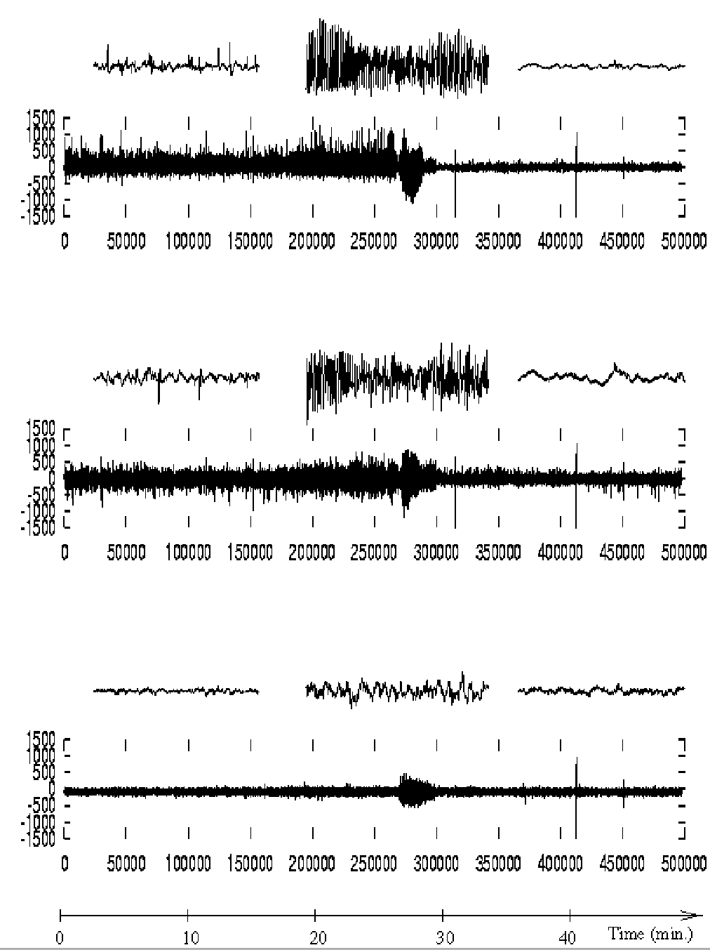
We will illustrate the result of the previous section by re-analyzing some of the same data used in [9]. The data correspond to an intracranial multichannel EEG recording of a patient with mesial temporal lobe epilepsy; it was sampled with 173 Hz and band pass filtered in the range $0.53-85$ Hz. In Fig. 1 we show EEG time sequences (500000 data points, approx. 48 min. of continuous recording) from three different recording sites prior to, during, and after an epileptic seizure. Seizure starts at about point 270000 (minute $26$ ) and lasts for 2 minutes. The recording sites are located nearest to the epileptogenic focus (upper trace; channel abbreviation: TBAR), adjacent to the focus (middle trace; channel abbreviation: TR), and on the non-affected brain hemisphere (lower trace, channel abbreviation: TBAL) To better visualize the dynamics, insets drawn on top of each signal show typical EEG sequences of 10 sec duration during the pre-seizure (left), seizure (middle), and the post-seizure stage (right).

3.2 Power spectrum

For a finite data set $x_{n}$ sampled at discrete times $t_{n}=n\Delta t,\;n=1,\ldots,N,\;T=N\Delta t$ , we denote by $X(\omega_{k})$ its discrete Fourier transform at $\omega_{k}=2\pi k/T$ , with $k=1,\ldots,N$ . We estimate the power spectrum as

S(\omega_{k})=C\;\sum_{n=-b}^{b}w(n)\cdot|X(\omega_{k+n})|^{2}

(14)

where $w(n)$ is a smoothing function of window size $B=2b+1$ , and $C$ is a normalization factor. As in ref. [9], a Bartlett-Priestley smoothing function was used

w(n)\propto\left\{\begin{array}[]{ll}[1-(n/b)^{2}]&|n|\leq b\\ 0&|n|>b\ \ \ .\par\end{array}\right.

(15)

As in [9] and for comparison purposes, we subdivide the data in (half overlapping) epochs of $T\simeq 24$ s ( $N=4096$ data points), and choose the window size of the Bartlett-Priestley function as $B=33$ . This window length corresponds to a frequency resolution of 0.042 Hz. In the following we consider the spectrum in the region $\omega<30$ Hz since no interesting activity occurs outside this band [4]. Moreover, since we are not interested in the absolute power, the normalization factor $C$ is adjusted such that the sum over all frequencies below 30 Hz gives unity.

3.3 Shannon entropy

Parts (a) - (c) of Figs. 2 - 4 show the EEG signals recorded at the three sites, contour plots of the corresponding normalized power spectra and time dependent estimates of the Shannon entropy $H$ . Prior to the seizure, power spectra exhibit an almost stable but spread frequency composition which is reflected in high values of $H$ .

When the seizure starts, the spectra in Figs. 2 and 3 are dominated by a single frequency component ( $\sim 7$ Hz). This is reflected in Fig. 2 by an abrupt decrease of $H$ by about 20%. Actually, the decrease is even more pronounced for smaller time windows, since the period of strong coherence is much shorter than 24 sec. As the seizure evolves, the dominant frequency decreases rapidly. This dynamics is characteristic of seizures originating from the mesial temporal lobe (see e.g. [13]) but it is not the only possible one [8]. The rise of $H$ in both Figs. 2 and 3 immediately before the final drop can partially be attributed to this fast change of dynamics. The estimated entropy is high during this phase because of several subsequently appearing frequencies in the same window. The following concentration of activity at lower frequencies finally leads to a decrease of $H$ . To a lesser degree this is also seen in Fig. 4. Within or close to the seizure generating area, $H$ remains small throughout the entire recorded post-seizure stage. Finally, it slowly increases towards values that compare to those obtained during the pre-seizure stage. Using a Shannon entropy defined from the wavelet transform, similar results were obtained in ref. [1] from an analysis of a scalp recorded seizure.

3.4 Kullback-Leibler entropy

The time courses of the K-L entropy $K(p|q)$ are shown in parts (d) of Figs. 2 - 4. As reference segments we used the signals from the pre-seizure stage consisting of 4096 data points and starting at $n=20480$ . The sensitivity (i.e. increase of $K(p|q)$ during the seizure relative to the background level) is notably improved when compared to that of the Shannon entropy. Background fluctuations during the pre-seizure stage only slightly affected $K(p|q)$ since pre-seizure power spectra from different windows are almost similar. Also, $K(p|q)$ proved nearly independent on the choice of the reference segment, as long as it was chosen from the pre-seizure stage.

As with the Shannon entropy we see in Figs. 2 and 3 a marked change at seizure onset due to a concentration of spectral power at frequencies $\sim 7$ Hz. $K(p|q)$ clearly detects this difference. It also detects the spectral difference when lower frequencies dominate in the post-seizure stage. But again the rapid frequency change after seizure onset is hard to distinguish from a broad band spectrum due to our somewhat large window size $T$ .

The last two parts of Figs. 2 - 4 show time courses of the K-L entropy and the renormalized entropy calculated using a reference segment with lowest Shannon entropy as was done by the authors of [9]. For Figs. 2 and 3 this was after the seizure (4096 data points starting at n=335872 and n=315392, resp.), while it was during the seizure for data shown in Fig. 4 (4096 data points starting at n=284672).

Here K-L and renormalized entropies give similar results. This illustrates the similarity between renormalized and K-L entropies as already pointed out in section 2. Differences with results in [9] can be attributed partly to differences in the exact choice of the reference segment. We see that peak values of $K(p|q)$ are larger than those based on calculations using a pre-seizure reference window. However, the relative increases over pre-seizure values are much less pronounced. Therefore, we consider post-seizure reference segments as not very useful for seizure detection. Moreover, post-seizure reference segments obviously can not be used in real-time applications. In addition, a post-seizure reference segment is not very reasonable physiologically. Immediately after a seizure, the state of the patient and, accordingly, the EEG are highly abnormal. Typically the post-seizure EEG exhibits slow fluctuations of high amplitude, sometimes superposed with high frequency activity (see Fig.1). This is obviously not an typical background EEG. Moreover, the post-seizure stage is often contaminated by artifacts, some of which are not as easily recognizable as those shown in Fig. 1.

We therefore disagree with the procedure proposed in ref. [9] of automatically choosing a reference as the segment with lowest entropy for each recording channel. Instead, we propose to choose a reference segment recorded during a state as “normal” as possible, i.e. far from a seizure (we should note, however, that there is still a lot of controversy in neurophysiology of what is considered to be “far”), free of artifacts and, if possible, free of abnormal alterations (admittedly, this is not always possible). Moreover, the reference segment should be exactly the same time interval for all channels. Otherwise comparisons between different recording sites are not reliable. Also, one might consider taking shorter time segments. This would of course enhance statistical fluctuations, but would allow better time resolution.

Even then it would be difficult to detect the recording site showing the very first sign of the seizure which is necessary for an exact focus localization. We verified this for windows down to 1.5 seconds (data not shown). This is in agreement with clinical experience which shows that the time scales relevant for this detection can be less than 1 sec. Because of these problems, the suggestions of [9] concerning clinical applications like seizure detection or localization of epileptic foci seem too optimistic.

4 Conclusion

The aim of the present paper was twofold. Firstly, we showed that “renormalized entropy”, a novel entropy measure for differences in probability distributions, is closely related to Kullback-Leibler entropy. We also argued that it is very unlikely that more information is obtained from the former than from the latter. Secondly, we checked recent claims that renormalized entropy (and thus also K-L entropy) is very useful in applications to intracranial EEGs from epilepsy patients. We found some of these claims to be unjustified. Nevertheless, the fact remains that K-L entropy applied to spectral distributions is a very promising tool which has not yet been studied much in this context. In fact, “abnormal” frequency patterns corresponding to epileptic seizures were better identified with K-L than with the Shannon entropy. While the present study was performed on a limited amount of data, we suggest K-L entropy to be an interesting tool for a more systematic study.

Finally, we point out that the K-L entropy can also be defined from other time-frequency distributions rather than the windowed Fourier transform. In particular, we consider wavelets as good candidates, since they have optimal resolution both in the time and the frequency range (see [6, 2] for theoretical background and [14, 17] for application to EEGs).

Acknowledgments: K.L. acknowledges support from the Deutsche Forschungsgemeinschaft.

References

[1] S. Blanco et al., Phys. Rev. E 57, 932 (1998).
[2] C. Chui, An introduction to wavelets (Academic Press, San Diego, 1992).
[3] G. Dumermuth G and L. Molinari, in Handbook of electroencephalography and clinical neurophysiology, Vol. I: Methods of analysis of brain electrical and magnetic signals, edited by A. Gevins and A. Rémond (Elsevier, Amsterdam, 1987) pp 85.
[4] J. Gotman, J.R. Ives, and P. Gloor, Electroencephalogr. Clin. Neurophysiol. 52, 626 (1981).
[5] R. Gray. Entropy and information theory (Springer-Verlag, New York, 1990).
[6] A. Grossmann and J. Morlet. SIAM J. Math. Anal. 15, 723 (1984).
[7] S. Guiasu, Information theory with applications (McGraw-Hill, New York, 1977).
[8] D. King and S. Spencer, J. Clin. Neurophysiol. 12, 32 (1995).
[9] K. Kopitzki, P.C. Warnke, and J. Timmer, Phys. Rev. E 58, 4859 (1998).
[10] J. Kurths et al., Chaos 5, 88 (1995).
[11] K. Lehnertz and C.E. Elger, Phys. Rev. Lett. 80, 5019 (1998).
[12] F.H. Lopes da Silva, in Electroencephalography: Basic Principles, Clinical Applications and Related Fields, edited by E. Niedermeyer and F. H. Lopes da Silva (Baltimore, Williams and Wilkins 3rd ed., 1993), pp 1097.
[13] R. Quian Quiroga et al., Electroencephalogr. Clin. Neurophysiol. 103, 434 (1997).
[14] R. Quian Quiroga and M. Schürmann, Clin. Neurophysiol. 110, 643 (1999).
[15] P. Saparin, A. Witt, J. Kurths, and V. Anishenko, Chaos, Solitons & Fractals 4, 1907 (1994)
[16] C.E. Shannon, Bell. Sys. Technol. J. 27, 379 (1948); 27, 623 (1948).
[17] S.J. Schiff, A. Aldrouby, M. Unser, and S. Sato, Electroencephalogr. Clin. Neurophysiol. 91, 442 (1994).
[18] A. Voss et al., Cardiovasc. Res. 31, 419 (1996)

Refer to caption — Figure 1: Intracranial EEG recordings [ $\mu$ V] prior, during, and after an epileptic seizure of right mesial temporal origin. Recordings were taken from within (electrode TBAR, upper plot) and adjacent to (electrode TR, middle plot) the seizure generating area as well as from the non-affected brain hemisphere (electrode TBAL, lower plot). See text for further details. The vertical lines at about 316000, 415000 and 451000 are due to artifacts in the recording. The data corresponding to these artifacts were not considered for further analysis.