Chance and Necessity in Evolution:
Lessons from
RNA
Thanks: Submitted to Physica D, Special
Issue on “Predictability: Quantifying Uncertainty in Models of
Complex Phenomena”
Abstract
The RNA folding map, understood as the relationship between sequences and secondary structures or shapes, exhibits robust statistical properties summarized by three notions: (1) the notion of a typical shape (that among all sequences of fixed length certain shapes are realized much more frequently than others), (2) the notion of shape space covering (that all typical shapes are realized in a small neighborhood of any random sequence), and (3) the notion of a neutral network (that sequences folding into the same typical shape form networks that percolate through sequence space).
The concept of a neutral network is particularly illuminating. Neutral networks loosen the requirements on the mutation rate for selection to remain effective. What needs to be preserved in a population is not a particular sequence, but rather a shape. This mandates a reformulation of the original (genotypic) error threshold in terms of a phenotypic error threshold confirming the intuition that more errors can be tolerated at higher degrees of neutrality.
With regard to adaptation, neutrality has two seemingly contradictory effects: It acts as a buffer against mutations ensuring that a phenotype is preserved. Yet it is deeply enabling, because it permits evolutionary change to occur by allowing the sequence context to vary silently until a single point mutation can become phenotypically consequential. Neutrality also influences predictability of adaptive trajectories in seemingly contradictory ways. On the one hand it increases the uncertainty of their genotypic trace. At the same time neutrality structures the access from one shape to another, thereby inducing a topology among RNA shapes which permits a distinction between continuous and discontinuous shape transformations. To the extent that adaptive trajectories must undergo such transformations, their phenotypic trace becomes more predictable.
Keywords:
Genotype-phenotype relation, intrinsic punctuation, molecular evolution, neutral networks, RNA secondary structureand
1 Introduction
In his provoking classic, Chance and Necessity [1], Jacques Monod expressed the belief that a “universal theory”, despite anticipating the appearance of certain classes of objects (such as galaxies, planetary systems, molecules, atoms, and the like), would not be able to account for the biosphere. The biosphere, Monod says, does not contain a predictable class of objects. Essential unpredictability from first principles does not imply that the biosphere is not explicable through these principles: biological objects have, in Monod’s words, “no obligation to exist, but they have the right to” ([1], p. 44). From a more rigorous point of view, the problem of predicting the class of objects that are outcomes of biological evolution, that is, species of organisms, is ill-posed as long as we lack a formal specification of this class [2]. A judgement on Monod’s position must, therefore, remain open for the time being.
While the selection pressures of natural evolution arise endogenously, artificial evolution allows to specify desired outcomes implicitly by fixing those pressures exogenously. For example, when RNA molecules are being intentionally evolved in the test tube to perform certain functions or to bind certain targets [3], an outcome is being implicitly specified in advance. The evolutionary problem then reduces to producing an actual RNA sequence folding into a shape implementing some prespecified properties. This is an adaptative process within a class of objects rather than the evolution of a class of objects (the process which Monod believed to be intrinsically unpredictable). Issues concerning the interplay of chance and necessity become smaller in scope but also better defined in the context of evolutionary adaptation. For example, is it predictable whether a desired outcome can be attained? And how predictable are adaptive trajectories given some level of abstraction?
When considering the production of antibodies during an immune response, Monod – like many – was puzzled by the effectiveness of adaptation as a search engine driven by selection and mutation alone. The puzzle about the effectiveness of adaptation is, as we shall argue, only apparent. It results from a misframing of the problem not unlike in the so-called Levinthal paradox [4] of protein folding, where the puzzle is (or rather, was) about how proteins can fold into their native structure despite a combinatorially large space of possible configurations. The Levinthal paradox has come to be recognized as resulting from a false dichotomy [5]: either the protein has to make an extensive search through its conformation space to find the lowest energy state (but then it should not fold within observable times), or it folds “down” some energy path (but then it should get stuck in a suboptimal trap). However, like protein folding, both the limitations and the opportunties for evolutionary adaptation derive from specific features of the “landscape” on which it occurs. The term landscape denotes here a space of appropriately weighted pertinent configurations - self-reproducing units and their fitness in the context of evolutionary adaptation, or molecular conformations and their (free) energy in the context of protein folding. Paths on such landscapes are not equiprobable. The stochastic dynamics of both the adaptive process (selection) and the folding process (least action) is guided by the landscape structure and explores only a tiny fraction of the possible configurations. This raises the issue about what exactly a “folding pathway” or an “evolutionary trajectory” consist in, and how well-defined they are. The ability to address the problem of predictability in adaptation depends on such a characterization.
Exploring the structure of landscapes is a very active area of empirical and theoretical research [6]. Despite the similarity of certain questions, and despite the fact that both processes crucially depend on special features of their landscapes, the analogies between folding of an individual molecule and evolutionary adaptation are limited. Landscapes underlying evolutionary processes differ fundamentally from energy landscapes, because biological entities are organized by a genotype-phenotype map. Replication and mutation occur at the level of the genotype, but the selective amplification of a genotype depends on the performance of its phenotype. This dichotomy wouldn’t be fundamental, if it were not for the fact that the genotype-phenotype map is characteristically many-to-one. The fact that many genotypes form the same phenotype enables (as it turns out) evolutionary adaptation to be successful. However, it also constitutes a major source of uncertainty in evolutionary trajectories.
The split into genotype and phenotype implies two different notions of “innovation”, and, hence, mandates care when speaking about “trajectories”. Should an evolutionary trajectory refer to a temporal succession of genotypes or of phenotypes? And how are the two related? It is important to realize here that genotypic and phenotypic innovation are not on an equal footing. A phenotype cannot be modified directly, but only indirectly through variation of its genotype. This indirection means that phenotypic innovation is mediated and, hence, biased by the genotype-phenotype map. Genetic mutations are random, but their consequences are far from random, as they depend on the context in which they are expressed. Assume, for example, that all one-error mutants of a gene are equally likely. Despite the absence of a bias at the genetic level, the resultant protein shapes would, however, occur with biased probabilities. Innovation is locally isotropic for genotypes, but the genotype-phenotype map channels phenotypic change along specific and much fewer directions. We should, therefore, expect regularities in the genotype-phenotype map to reduce the “phenotypic uncertainty” of evolutionary trajectories as compared to their “genotypic uncertainty”.
Imagine a game that is played on two boards, the g(enotype)-board and the p(henotype)-board. The game allows the player to make local moves on the g-board only, while the actual pay-off is determined by moves on the p-board. Some unknown machinery transduces the g-board-moves into p-board-moves. Even if the g-board-moves were entirely random, an observer of the p-board would pick up statistical regularities reflecting the transducing mechanism. Suppose further that an “invisible hand” holds the player’s stone on the p-board fixed. The transducing machine then acts back to confine the player to a subset of moves on the g-board which are compatible with the stone’s fixed position on the p-board. We call these moves neutral, as they don’t change pay-off. The set of squares on the g-board that the player can access by moving under this constraint we call a neutral network. Imagine now the invisible hand softening its grip to allow moves on the p-board that do not decrease pay-off (such as selection). If none of the neighboring squares of the player’s position on the g-board yields a pay-off increase, the player won’t be stuck, as moves to neighboring neutral squares are still an option. Their neighbors might trigger pay-off increasing moves on the p-board. As long as the stone on the p-board remains in a fixed position, an observer of the p-board may conclude that nothing is happening, and an observer of the g-board notes only “more of the same” as the pay-off stays constant. The point, however, is that by moving neutrally something does vary: the potential for change. Without neutrality the game would quickly become stuck in a suboptimal trap, and the “evolutionary Levinthal paradox” would be a real one. However, with a sufficient degree of neutrality the very notion of a “trap” looses its relevance, as “lateral” (fitness-neutral) moves change opportunities at no cost.
In this contribution we review work on the most realistic molecular model for the genotype-phenotype dichotomy available to date. RNA unites both the genotypic and the phenotypic level in a single molecular object. The genotype is the sequence which can be replicated in the test tube by suitable enzymes, and the phenotype is the structure which can be subject to selection. We will summarize the salient properties of the folding relation between sequences and structures. This sets the stage for discussing some central aspects of evolutionary dynamics in models of evolving populations of RNA molecules. We shall focus in particular on an emerging notion of “evolutionary trajectory” which is far from being fully understood but which invites deeper investigation. This will prompt us to think about what is and what is not predictable.
The main take-home should be an appreciation for the central and apparently paradoxical role played by neutrality. On the one hand, neutrality (or redundancy, for that matter) is conservative, because it buffers against inevitable mutations ensuring that “nothing happens”, that once attained success is not too easily lost. Yet at the same time neutrality is deeply enabling, because it permits evolutionary change to occur by allowing the sequence context to vary until a mutation can become phenotypically consequential. In the dynamics picture neutrality sets the stage for adaptation in jumps, that is, intrinsic punctuation. But neutrality does more: it endows the set of phenotypes with a topological structure. A many-to-one map induces equivalence classes of genotypes labelled by phenotypes. Nearness (or accessibility) between phenotypes, then, should be defined to reflect nearness between equivalence classes of genotypes. Once we possess a topology we can start thinking about whether and when evolutionary trajectories are “discontinuous”. While chance events will not allow to predict when a discontinuity will happen, the topology enables the prediction of what class of changes will be involved. We conclude by placing the lessons learned from RNA into the larger perspective of evolution.
2 RNA: an experimental and theoretical model system
Understanding how notions like “evolutionary path” and “continuity” (or “discontinuity”) are shaped by adaptive landscapes, requires a model system that captures essential properties of the relationship between genotype and phenotype. Since we don’t know these properties a priori, any theoretical model must have a firm empirical grounding to begin with. In addition to being computationally tractable, the system should also be a laboratory model of evolutionary adaptation. This excludes multicellular organisms, since their complexity does not permit at the present state of knowledge an empirical and theoretical tracking of how the genotype-phenotype relation (i.e., development) plays out during an evolution experiment in the laboratory. Prokaryotic organisms don’t undergo development but the cellular metabolism is still too complex to be included in a genotype-phenotype map. Settling for less than organismal complexity, we arrive at RNA as the simplest non-trivial molecular system fulfilling “ideal model” requirements.
What makes RNA unique is the simultaneous presence of both levels, genotype and phenotype, in a single molecule. RNA molecules are heteropolymers of (predominantly) four units called ribonucleotides. Ribonucleotides have the ribose phosphate in common, but differ in the base attached to the sugar. RNA molecules are represented as sequences over a four letter alphabet, with each letter standing for a particular base - A for adenine, U for uracil, C for cytosine, and G for guanine. Interactions mediated by hydrogen bond patterns give rise to a stereoselective recognition between specific pairs of bases - AU and GC. This specific base pairing enables an RNA sequence to be copied via a complementary negative, and hence to function as a genotype. At the same time it enables segments of a sequence to pair with other segments within the same sequence, causing the sequence to fold back on itself into a structure. (In the formation of intramolecular structure GU pairs are possible as well.) This structure mediates the chemical interactions of the sequence, and hence constitutes its phenotype.
“Structure” can be seen at many levels of resolution, extending from atomic coordinates to the mean radius of gyration. This raises the question of what constitutes a relevant level of structure resolution for understanding adaptation. We take a pragmatic stance here, but we shall return to this issue in conclusion. On the theoretical side we require computability from the sequence, and on the empirical side we require usefulness in interpreting molecular function and evolutionary data. This leaves us with an empirically well established level of resolution known as secondary structure. The secondary structure of an RNA molecule refers to a topology of binary contacts arising from specific base pairing, rather than a geometry cast in terms of coordinates and distances (Figure 1). The driving force behind secondary structure formation is the stacking between contiguous base pairs. The formation of an energetically favorable paired (or double-stranded) region implies, however, the formation of an energetically unfavorable loop. This “frustrated” energetics leads to a vast combinatorics of stack and loop arrangements spanning the structural repertoire of an individual RNA sequence.

A secondary structure can be conveniently discretized as a graph representing the pattern of base pair contacts (Figure 1). The nodes of the graph represent bases at positions along a sequence of length . The set of edges consists of two parts. One is common to all secondary structure graphs, and represents the covalent backbone connecting node with node , . The other part is the secondary structure proper, and consists of a set of edges , , representing admissible hydrogen bonds between the bases at positions and . The set has to satisfy two conditions: (i) every edge in connects a node to at most one other node, and (ii) if both and are in , then implies that . Failure to meet condition (ii) results in interactions (pseudoknots) considered as belonging to the next - the tertiary - level of structure. Both conditions distinguish RNA structure from protein structure, in particular condition (i) which builds RNA secondary structure exclusively from binary interactions. We use a picture of the graph as the visually most immediate representation of a secondary structure. It proves convenient to also use a line oriented representation, such as “((((.(((...))).(((...))).))))”, where a dot stands for an unpaired position, and a pair of matching parentheses indicates positions that are paired with one another.
Observe that the building blocks of a secondary structure are classes of loops (Figure 2): a hairpin loop is delimited by one base pair which encloses a number of unpaired positions, a stack is delimited by two base pairs and has no unpaired positions, while an internal loop is delimited by two base pairs that enclose unpaired positions. An internal loop is called a bulge, if either side has no unpaired positions. Finally, the class of multiloops consists of loops delimited by more than two base pairs. A position that does not belong to any loop class is called external, such as free ends or joints between loops (see Figure 1). The importance of these loop classes derives from the reasonable assumption that the overall energy of a secondary structure is the sum of its loop energies, and from the fact that their free energies have been measured and tabulated [7, 8, 9, 10] as a function of loop size and the nature of the delimiting base pairs.

Secondary structure graphs are formal combinatorial objects which can be subject to mathematical treatment (they can be counted, for instance). Of particular interest are secondary structures possessing some extremal property with respect to a given sequence, such as minimizing the free energy. The theoretical importance of RNA as a model system for sequence-structure relations in biopolymers lies in the fact that structures of this kind can be computed by dynamic programming [11, 12, 13, 14, 15]. This method produces a single structure that minimizes free energy. Following an idea by Waterman [16] we have recently extended the standard RNA folding algorithm to compute all structures within some energy range above the minimum free energy [17]. However, for the present discussion the minimum free energy structure will suffice, and we shall consider it to be the phenotype of an RNA sequence.
The secondary structure is not just an utter abstraction, but it provides both geometrically and thermodynamically a scaffold for the tertiary structure. Its free energy accounts for a large share of the overall free energy of the full structure. This linkage puts the secondary structure in correspondence with functional properties of the tertiary structure. Consequently, selection pressures (and hence functional elements) become observable at the secondary structure level in terms of conserved base pairs.
The extremely reduced amplification time and the minimal complexity of the phenotype make RNA a tractable laboratory model. RNA molecules can be evolved in the test tube using a variety of techniques for amplification, variation and selection. In fact, such experiments have shown that evolutionary optimization of RNA properties in the test tube occurs readily and effectively. Examples are the optimization of replicative efficiency [18, 19], the production of RNA molecules binding optimally to prespecified target molecules by means of the SELEX technique [20, 21], evolutionary induced changes in the activity and specificity of catalytic RNA molecules [22] (so-called ribozymes), and the evolutionary design of ribozymes with new functions [23, 24]. Often the interpretation of such experiments occurs by computing the secondary structure and placing it in relation to molecular performance.
Until now the bulk of empirical interest has been directed at the outcomes of evolutionary test tube experiments. However, we shall take here outcomes for granted, and focus instead on dynamics and paths toward outcomes. These aspects hold the key for understanding why (and which) desired outcomes can be achieved at all. An emerging evolutionary technology will depend on a comprehensive dynamical theory of molecular adaptation, much like chemical engineering depends on chemical kinetics.
3 Characteristic features of the RNA folding map
The first computer experiments on the adaptive dynamics of replicating and mutating RNA populations [25] were very encouraging, but they also made it clear that to understand adaptive dynamics, we must first understand the features of the landscape induced by RNA folding. The term “landscape” emphasizes the folding map as a function from a space of sequences into a space of structures (with possibly a further assignment of numerical values to each structure). The set of RNA sequences of length comprises possible variations that are organized into a metric space by a natural distance measure reflecting the allowed physical interconversions of sequences. The Hamming distance is a natural distance measure, if only point mutations are allowed. It counts the number of positions in which two sequences differ, that is, the minimum number of point mutations required to convert one sequence into the other. In the case of a two-letter alphabet this space is the well-known -dimensional hypercube. The set of secondary structures can also be made into a metric space. Structure distance functions are typically based on some notion of minimum edit cost for transforming one structure into another, such as the Hamming distance or the base pair distance [26] defined on the dot/parentheses representation of secondary structures, or the tree-edit-distance [27]. If the structure space is metric, it becomes possible to assess the “ruggedness” of the landscape by autocorrelation functions [28]. However, it is not always necessary or useful to think of the set of secondary structures as a metric space. In section 5 we shall think of it as a topological space.
Our interest is thus primarily aimed at extracting robust statistical properties pertaining to the mapping as a whole. Although we use state of the art algorithms [14, 26, 29] that are routinely applied to predict the secondary structure of sequences occurring naturally or having evolved in the laboratory, our main focus is not the accurate prediction of a structure from a particular sequence. (This would anyway require an integration with data from phylogenetic comparison.) We seek qualitative and generic features of adaptive dynamics in RNA, and these should not depend on whether the employed algorithms reproduce the fine details of the actual secondary structure in a particular instance. Rather, we rely on the fact that the employed algorithms are sufficiently mature that they correctly capture the logic and basic energetics of constrained base-pair optimization inherent in RNA folding. In fact, the generic features of the folding map summarized below have been found to be insensitive to the choice of structure formation criteria, such as minimizing free energy, maximizing base pairing, or kinetic folding. They also are numerically robust to variations in the set of empirical energy parameters or the thermodynamic level of description (one minimum free energy structure versus the Boltzmann ensemble for a given sequence) [30]. It is encouraging that similar properties have also been recently discovered in lattice models of protein folding [31, 32, 33]. For the remainder of this paper we shall - for the sake of brevity - refer to secondary structures simply as “shapes”.
A systematic study of the mapping from RNA sequences to shapes was based on the statistics of appropriately chosen samples [27, 28, 34] as well as on the exhaustive folding of all sequences of a given length [35, 36]. The regularities found depend on two simple and fundamental facts. First, both the sequence and the shape space are very high dimensional spaces (forget three-dimensional caricatures), and, second, the sequence space is substantially larger than the shape space. An upper bound along the lines of [37] yields only shapes vis à vis sequences [38]. It is clear that the mapping from sequences to shapes is significantly many-to-one, even if the alphabet were binary. These, then, are the major generic properties that were found:
Property 1 (“typical shapes”) states that some shapes are supported by significantly larger equivalence classes of sequences (i.e., occur more frequently) than others. These relatively few typical shapes are set apart from many rare shapes which can hardly play a role in evolution. The property of being ‘‘typical’’ is made more precise by the observation that in the limit of long chains the fraction of such shapes tends to zero (their number grows nevertheless exponentially), while the fraction of sequences folding into them tends to one.11 1 This asymptotic condition for “typical” is fulfilled by a whole class of definitions. A simple and straightforward one is that of a so-called “common shape” which refers to a shape formed by more sequences than the average given by the number of sequences divided by the number of realized shapes [39]. A numerical example may help: The space of GC-only sequences of length contains sequences folding into structures of which () classify as typical (in the sense of “common”, see footnote 1). In this case of all sequences fold into these shapes. Property 1 also implies that any statistical statement we make about the folding map, and a fortiori about adaptive dynamics, can only hold for the set of typical shapes.
Property 2 (“neutral networks”) is a statement about the connectedness in sequence space of sequences folding into the same shape. Typical shapes are characterized by a high degree of neutrality expressed as the average fraction of nearest neighbors of a sequence possessing a typical shape that retain that shape. A large enough degree of neutrality, expressed as the mean fraction of neutral neighbors with Hamming distance one, leads to percolation in sequence space, that is, to the existence of extended neutral networks connecting sequences with the same shape by one or at most two point mutations (Figure 3).

Property 3 (“shape space covering”) is a statement about the mutual entanglement of neutral networks belonging to different shapes. All typical shapes are realized within a small neighborhood (compared to sequence length) of any arbitrarily chosen sequence (Figure 4). For example, 15 mutations are sufficient on average for a chain of length to find at least one instance of every typical shape.

These statistical properties, in particular neutral networks, have led to a mathematical model based on percolation in random graphs [40]. There is no doubt that neutrality is an essential feature of adaptive topographies. It is, therefore, crucial that models of adaptive landscapes take neutrality into account, see for example [41, 42, 43, 44, 45, 46]. We shall explore some of its effects in the following two sections.
4 Error propagation in genotype and phenotype populations
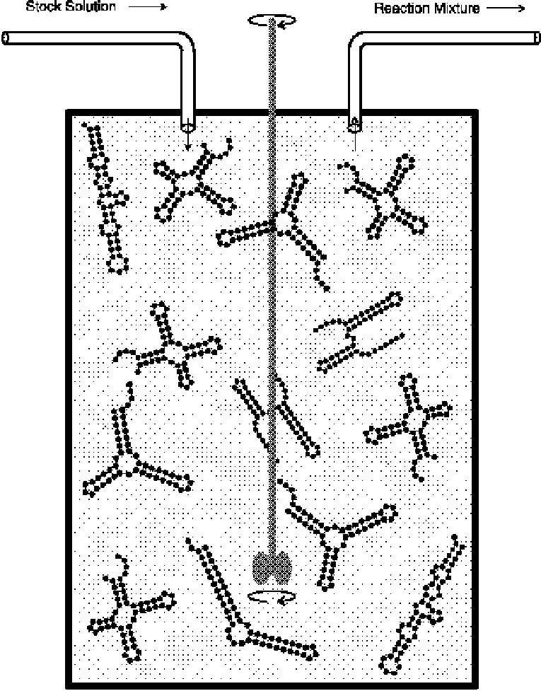
The evolutionary dynamics of molecules based on replication, mutation and selection induced by a constant population size in a flow reactor has been analyzed in terms of chemical reaction kinetics by Manfred Eigen [47], and was further developed in subsequent studies [48, 49]. Faithful copying and mutation are treated on an equal footing by viewing the replication of an RNA sequence as a branching reaction with many channels. In principle every sequence can be obtained as a mutant from every sequence (although the probabilities vary dramatically). The materials consumed by RNA synthesis are replenished by a continuous flow in a reactor resembling a chemostat for bacterial cultures (Figure 5). The character of the dynamics of a sequence population depends critically on two factors, the accuracy of replication which governs the “width” of individual reaction channels and the degree of neutrality - a property of the genotype-phenotype map - which governs the decoupling of the propagation of a given phenotype from the propagation of its underlying genotypes. The presence of neutrality mandates a distinction between a genotypic and a phenotypic error threshold [50]. The point of this section is to caricature the essence of this distinction in a very simple way. This will set the stage for discussing trajectories as influenced by the RNA genotype-phenotype map in section 5.
Selection dynamics in sequence populations can be described by ordinary differential equations. The variable , denotes the relative frequency of a sequence type (i.e., genotype) Ii of length . For the sake of brevity we shall overload the word “sequence” to mean an individual instance or a type, depending on context. Since frequencies are normalized, we have . We further denote the population size with , and the number of possible sequences with . Let the rate constants for replication and degradation of sequence Ii be and , respectively. The time dependence of the sequence distribution is then described by the kinetic equations
| (1) |
It has been assumed for simplicity that replication is direct, rather than proceeding through a complementary negative, as the base pairing rules would require (see [47, 49] for details). The width of the reaction channel from sequence Ii to sequence Ij is given by the mutation matrix . denotes the likelihood that a replication of sequence Ii yields sequence Ij, and the diagonal element is the fraction of correct replicas synthesized on template Ii. To fulfill , the reactor outflow matches exactly the average productivity, . When degradation is negligible, as in the test tube evolution of RNA molecules or when all degradation rates are essentially the same, , degradation has no influence on the selection dynamics and can be neglected. In this case the quantities which determine the selection dynamics are given by the so-called value matrix: , whose diagonal elements were called selective values.
The selective value of sequence Ii amounts to its fitness in the case of vanishing mutational backflow, . Under these conditions the sequence Im with the maximal selective value
| (2) |
dominates a population in selection equilibrium, and is called the master sequence.
The term quasispecies was introduced for the stationary sequence distribution, whose values are computed as the solutions of , from the eigenvalue problem [51, 52]
| (3) |
where denotes the unit matrix, an eigenvalue and the corresponding eigenvector.
4.1 Genotypic error threshold
To understand the difference between genotypic and phenotypic error thresholds, we consider the so-called single peak landscape which assigns a higher replication rate to the master and identical values to all others, and , where is the superiority of the master sequence. The assumption behind the single peak landscape is to lump together all mutants into a cloud with average fitness. The relative population frequency of the cloud is simply , and the replication-mutation problem boils down to an exercise in one variable, , the frequency of the master. The approach has something in common with the mean field approximation often used in physics, since the mutant cloud can be characterized by “mean except the master” properties. For example, the “mean except the master” replication rate constant . The superiority then reads: .
Neglecting muational backflow we can readily compute the stationary frequency of the master sequence in a “zeroth-order” approximation:
| (4) |
In this expression the master sequence vanishes at some finite replication accuracy, . A non-zero stationary frequency of the master, that is, its indefinite propagation, thus requires . This is the so-called error threshold condition. It is illuminating to introduce a simple model for the elements of the mutation matrix, called uniform error rate approximation [48]. It assumes the existence of a per nucleotide mutation probability that is independent of the nature of a nucleotide and its position in the sequence. In terms of the single digit accuracy (the mean fraction of correctly incorporated nucleotides) the elements of the mutation matrix for a sequence of length take the form:
| (5) |
with being the Hamming distance (i.e., the number of mismatches) between two sequences Ii and Ij. The critical condition occurs at . The replication accuracy of RNA viruses was indeed found to occur near this critical value [53, 54].
To study stochastic features of the population dynamics around the critical replication accuracy, the replication-mutation system has been modeled by a multitype branching process [55]. The main result of this study was the derivation of an expression for the probability of survival to infinite time for the master sequence and its mutants. In the regime of sufficiently accurate replication the survival probability is non-zero and decreases with increasing error rate. At the critical accuracy this probability becomes zero, which implies that all molecular species currently in the population will die out in finite time and new variants will replace them. This scenario is tantamount to migration of the population through sequence space.
Further details of the population structure require consideration of the mutational backflow (and thus a solution to the eigenvalue problem, equation 3). The two eigenvectors associated with the two largest eigenvalues at represent the quasispecies and the uniform distribution, , respectively. These eigenvectors show avoided crossing at the critical accuracy [56]. Since the off-diagonal elements are small and decrease further with increasing chain length , the zeroth order approximation to the frequency of the master is fairly good (), and the transition from the quasispecies to the uniform distribution is sharp [49, 57]. Obviously, the deterministic approach becomes meaningless at accuracies below threshold, when the uniform distribution, , implies less than a single molecule for each variant. This is already the case for fairly small chain lengths of , when the population size required for the deterministic approach () exceeds the feasible sizes realizable in test tube evolution experiments ().
4.2 Phenotypic error threshold
In the case of neutrality the superiority of the master becomes , which pushes the error threshold towards absolute replication accuracy, , and the deterministic model must fail. Any sequence on a neutral network is inevitably lost at non-zero mutation rates, but the phenotype associated with that network may nevertheless persist. Neutrality, thus, shifts the focus from genotypes to phenotypes, suggesting a treatment where phenotypes become the relevant units by lumping together sequences with equal phenotype. Given possible phenotypes, we define new aggregate variables, (), by collecting the set of sequences with given phenotype and replication rate (latin letters refer to sequences and greek ones to phenotypes):
| (6) |
with . In analogy to the previous treatment we call the phenotype with maximal fitness the master phenoptype. Since we are heading again for a zeroth-order approximation, we only consider the master phenotype. Without loss of generality we index the sequence types possessing the master phenotype from to , so that . This yields the kinetic equations for the set of sequences with master phenotype:
| (7) |
The mean excess productivity of the population is, of course, independent of the choice of variables:
| (8) |
To derive a suitable expression for the phenotypic error threshold, we split the mutational backflow into two contributions, (i) a mutational backflow within the neutral network of the master phenotype and (ii) a mutational backflow on to the master network from sequences not belonging to it:
| (9) |
We approximate the within-network backflow by assuming that a sequence on the network has a constant fraction of neutral neighbors. We further assume equal mutation rates () on the master network and find:
| (10) | |||||
| (11) |
To keep things comparable, we make the same approximation as in the genotypic error threshold and neglect mutational backflow from other networks () on to the master network. The kinetic equation (7) for the master phenotype can now be written as:
| (12) |
where expresses an effective replication accuracy of the master network as such:
| (13) |
Proceeding in complete analogy with the derivation of the genotypic error threshold, we find
| (14) |
where is the superiority of the master phenotype. The uniform error rate model yields for the stationary frequency of the master phenotype:
| (15) |
The “zeroth-order” approximation for the phenotypic error threshold () now becomes:
| (16) |
The function is illustrated in Figure 6. In the limit of no neutrality, , both phenotypic and genotypic error threshold are the same, . In the limit of “extensive” neutrality, , the minimal replication accuracy approaches zero. This means that when the degree of neutrality exceeds the reciprocal superiority, the master phenotype is never lost from the population, no matter what the mutation rate is.

This section’s goal was to show that neutrality leads to populations whose sequences drift randomly on the neutral network of the master phenotype, or, for that matter, any temporary most fit phenotype [50]. Even if the sequence distribution drifts, the phenotype is maintained. However, if the replication accuracy falls below a critical minimum value - the phenotypic error threshold - the population drifts through both sequence and shape space. Interestingly, if the neutrality associated with a phenotype exceeds a certain level, the phenotypic error threshold disappears, and that phenotype cannot be lost from the population at any mutation rate.
Neutrality suggests a reformulation of Eigen’s original kinetic description and its stochastic versions in terms of neutral networks as the units of aggregation. The switch in variables is complicated by the fact that the sequence mutation matrix must be translated into a “mutation” matrix which refers to transitions between neutral networks, i.e. phenotypes. This is where we heavily glossed over in this section, since it requires an understanding of the sense in which networks are “adjacent” to one another. One quite fruitful approach is to define prototype landscapes [40, 44, 45, 58], another is to analyze this adjacency relation in the concrete case of RNA [59], and to extract regularities which may guide the design of model landscapes. We shall turn to this in the next section.
5 Adaptive paths and intrinsic punctuation
In this section we lay some groundwork for framing adaptive trajectories in evolving RNA populations. To this end we must first understand the organization of RNA shape space.
5.1 The topology of RNA shape space
We have seen in section 4 that neutrality loosens the requirements on the replication accuracy for selection to remain effective. This increases the uncertainity of adaptive trajectories through sequence space, as populations with tiny sizes compared to the number of all possible sequences undergo neutral diffusion. At the same time, however, adaptive trajectories are subject to quite specific constraints. To see this informally, consider that for phenotypes to adapt, transitions between neutral genotype networks (that is, phenotypes) must occur. Some transitions are easy, others not. If the replication accuracy is sufficiently high, so that most mutants are one-error mutants, the degree to which a transition from one network to another is easy depends on how much of their boundary both have in common. This suggests defining a nearness relation between phenotypes (a topology) based on the extent to which their corresponding neutral networks are adjacent in genotype space [59, 60]. Notice that a so defined nearness relation is independent of a notion of similarity between phenotypes. Transitions between neutral networks sharing a small fraction of their boundary will, then, act as bottlenecks, and the uncertainty of adaptive trajectories will be reduced to the extent that they must pass such bottlenecks. If we can characterize the set of possible bottlenecks, we should be able to predict a class of phenotype transformations that any adaptive trajectory must go through, although we may not be able to predict the exact phenotypes involved or their temporal succession. We shall call this class a class of “way points”.
In RNA, as in many biological situations, there are two mappings involved which need to be kept distinct: the mapping from genotype to phenotype and the mapping from phenotype to fitness. Both are typically many-to-one and induce neutrality. However, the map from phenotypes to fitness depends on the (exogenous or endogenous) selection criteria, while at least in the case of RNA folding the genotype to phenotype map does not. Because the class of phenotype transformations that we are seeking is an intrinsic property of a given genotype-phenotype relation, it constrains adaptive trajectories in a fashion that holds under any (non-trivial) fitness assignment.
We shall now make these intuitions precise, and characterize the class of way points for RNA secondary structures based on a statistical analysis of the folding map. We then juxtapose these results with adaptive trajectories obtained from simulating a population of RNA sequences that replicate and mutate in a flow reactor under selection.
A particular adaptive path consists of a temporal succession of sequences and their associated shapes. We refer to the temporal series of shapes as the phenotypic trace. Whether a shape succeeds a shape will be strongly influenced by fitness. Yet for this to be an issue at all must first occur somehow, that is, must be accessible from by a mutation of ’s sequence. If is very likely to be accessible from , we shall call “near” . In the case of neutrality a shape is realized by a large set of sequences, and a robust notion of accessibility then comes to mean that must arise from with a high probability when averaged over all sequences folding into . Only then are the shapes in the phenotypic neighborhood of a robust property of itself, independent of a particular sequence.
This notion of neighborhood is illustrated by considering a tRNA-like shape of length 76 (inset of Figure 7). A sample of the many sequences folding into this shape was obtained by an inverse folding procedure [26] available with the Vienna RNA package [29]. For every sequence in the sample we compute all shapes realized in its sequence space neighborhood, consisting of all one-error mutants. From this data we determine the fraction of sequence neighborhoods in which a particular mutant shape appeared at least once. The totality of these mutant shapes, irrespective of how often they occurred, is termed the shape space boundary of the tRNA shape.
When rank-ordering the boundary shapes with decreasing frequency, we obtain Figure 7. The most salient feature is a marked change in the scaling exponent, suggesting a natural cut-off point for the definition of neighborhood. In the present case, the high frequency range comprises some 20 shapes, which we define to be near the tRNA shape [59]. These shapes constitute the characteristic set of the tRNA, that is, its most specific neighborhood. The topmost 12 shapes are shown in Figure 8, and exhibit two properties we found to hold for all shapes whose neighborhoods we studied. First, most shapes in the characteristic set of a shape are highly similar to , typically differing in a stack size by single base pairs. Second, some shapes, such as tRNA8 (the shape ranked 8th in Figure 8), differ by the loss of an entire stack. The latter finding illustrates that nearness of a shape to another does not imply their similarity. More importantly, it illustrates that nearness is not a symmetric relation. In fact, the tRNA shape was not found in the characteristic set of the tRNA8, and it did not even occur in its boundary sample. Not surprisingly, the destruction of a structural element (in a random sequence bearing it) through a single point mutation is easier than its creation. While the high frequency of the event is surprising, it is ultimately a consequence of the average base pair composition of stacks and the markedly different stacking energies of AU and GC base pairs [59].


The nearness relation developed here defines a topology on the set of RNA shapes. We call a transition from shape to a near shape continuous (in the spirit of topology), if that transition is caused by a single point mutation (since in that case the sequence of is in the obvious sense near the sequence of ).
Generalizing from this example, we can characterize continuous transformations as those structural rearrangements which fine tune a shape architecture in a sequential fashion by lengthening or shortening stacks, or which destroy a stack element and the loop implied by it (Figure 9). This leaves the discontinuous transformations characterized by the two remaining possible structural changes: (i) the creation of a long stack in a single step, and (ii) generalized shifts (see Figure 9). As an example of a shift consider one strand of a stacked region sliding past the other by a few positions (simple shift). Notice here that structural similarity does not imply nearness. Both types of discontinuous transformations require the synchronous participation of several bases (or base pairs) in a fashion that cannot be sequentialized on thermodynamic grounds. An example for a discontinuous transition of type (i) is the formation of a multiloop (a loop issuing more than two stacking regions). Generally, the free energy gain upon formation of a stack must offset the free energy loss from the loop caused by it. A stack closing a multiloop must, therefore, come into existence with some minimum length (typically more than 5 bp) in a single step. Likewise, the discontinuity of generalized shifts (type ii) has thermodynamic and structural origins. Shifting a stack by shifting its base pairs in random order would cause energetically unfavorable internal loops as well as severe sterical conflicts, besides violating the formal no-knot condition (section 2). As a consequence, the shifting of a stack requires that all base pairs move synchronously.

We may visualize the neighborhood structure on the set of all shapes (the topology) as a directed graph. Each shape is represented by a node. Directed edges fan out from a node to the nodes in its characteristic set. We can think of a continuous transformation of shape into a shape that is not nearby as a path from to following the direction of the edges. Discontinuous transformations are transitions between disconnected components of the graph.
5.2 Adaptive dynamics in RNA
We next discuss how the topology of RNA shape space shapes adaptive histories. Our simulation of replicating and mutating RNA populations is cast in terms of stochastic chemical kinetics [61, 62], and represents a continuous time model of Spiegelman’s classic serial transfer experiments [19, 63]. It’s implementation is described elsewhere [25, 64]. In the laboratory a goal might be to find an RNA aptamer binding to some molecule [65], and the evolutionary end product is typically unknown. In principle one can think of the end product as some shape that is specified implicitly by the imposed selection criterion. Since our intent is to study evolutionary trajectories rather than end products, we short cut by simply defining a target shape in advance. We then assume the replication rate constant of a sequence to be a function of the distance between its shape and the target. Given a distance measure , a shape replicates faster, the more it resembles the target. In all simulations reported here, the replication rate of a sequence Ii of length with shape at distance from a target shape is given by . Using an exponential or a linear function did not make any difference with regard to the issues we are interested in. The error rate was per nucleotide. At this rate, the difference between parent and a mutant offspring is mostly one point mutation, and the topology described above applies. In the examples reported here the target shape is a tRNA clover leaf, and the distance between shapes is measured as the Hamming distance between their line oriented representations cast in terms of dots and parentheses (see section 2).
Figure 10 and Figure 11 both show the approach toward the target shape as indicated by the average Hamming distance in the population (inversely related to fitness, black curve). Aside from a short initial phase, the entire history is dominated by steps, that is, flat periods of no apparent adaptive progress, interrupted by sudden improvements toward the target. The initial relaxation period is understood by considering that many modifications of a random initial shape increase its similarity to any randomly chosen target. Beyond this phase, however, adaptation becomes much harder, and the character of adaptive dynamics changes.


By adaptive trajectory we mean something like a path taken by the population as a whole (caveats below), rather than a single lineage. We refer to its projection on shape space as its phenotypic trace. In a simulation of this kind one has to cope with a huge amount of data, and one possibility of obtaining an approximation to the phenotypic trace of an adaptive trajectory is to record only data about mutation events that generate an “innovation”, that is, a shape which is new in the population at the time of its appearance. This does not neccesarily imply that the shape hasn’t been in the population in the past; it could have become extinct at some earlier time, being “rediscovered” at time . For each shape innovation we record entry times, , and exit (extinction) times . This yields for each shape ever seen during the adaptive process a set of “presence intervals” , marking the presence of shape in the system’s history. After the target has been found (or the simulation has been stopped), we trace back through the history data in the following way. Each presence interval of has a unique ancestor with shape which spawned that interval at time , meaning that a sequence folding into produced at time a mutant which folded into , and was not in the population at that time. Let be the target shape, and the time of its first appearance (the beginning of its presence interval). Let the shape from which was derived at time be . In the set there is a unique presence interval containing the time instant , and we proceed searching for the unique ancestor of . Upon repeating this procedure we eventually end up at one of the initial shapes (see Figure 12). At this point we have reconstructed a succession of shapes connecting an initially present shape with the target (or final) shape . This chain is uninterrupted in time, in the sense that for every , is ancestor of and there exists a pair with . The chain depends on the presence interval of the final shape from where the trace starts, but it is unique for that interval. Typically we are interested in the chain that originates in the first instance of the target, and call it the “relay series”.

Figures 13 and 14 show the complete relay series for the computer simulations reported in Figures 10 and 11, respectively. While the discontinuities in the fitness trace of Figures 10 and 11 are apparent, it is their comparison with the shape discontinuities along the relay series which yields insight. The result is that fitness triggered selection events do not always line up with shape transformations that are discontinuous in the sense of the previously defined topology. In Figure 10, events (a) and (b) are rapid successions of continuous transitions shortening and elongating stacks by single base pairs. This shows that sudden changes in fitness do not imply discontinuous phenotypic transformations. The reverse isn’t true either, as shown by the discontinuous shift event (c) which is silent in terms of fitness. All remaining fitness changes do, however, coincide with discontinuous shape transformations. These are the simple shift events (e), (g), (h), (i), the double flip (d), and the flip (f). Similar observations hold for Figure 11. Here we have an initial phase of rapid improvments (a), four simple shift events (b), (f), (g), (h), a flip (c), a double flip (e) as well as a “silent shift” (d) being a neutral discontinuous transitions, that is, a shift which does not change fitness.


To trigger a generalized shift or a multiloop closure by a single point mutation puts constraints on the required sequence context, making such sequences rare. When a shape is under strong selection, neutral drift is the only means for eventually producing such a sequence [50, 66]. This is why discontinuous transitions are preceded by extended periods of neutral drift in Figures 10 and 11.
It is important to realize that the present reconstruction of an adaptive trajectory is not identical to the succession of shapes associated with the actual lineage of sequences that led to the target. The relay series reports for all from start to target that (some sequence folding into) shape was sufficient for giving rise to a new shape . In the actual successful lineage may not have arisen from the first sequence with shape ; for that matter, it may not even have arisen from any sequence with shape . (Sequences with other shapes may also have produced , while was already present in the population.) In sum, the relay series is a fictitious path. The point is that it is a possible path and a very useful representative of the ensemble of paths shown to be possible by a population in a particular adaptive history. Let us explain. At any given time a population contains a number of individuals (instances) for each of the sequence types present. Each individual has its unique lineage of ancestors all the way back to the initial individuals. At the level of individuals there would obviously be only one successful lineage or causal path to the first appearance of the target. However, it makes sense not to distinguish among identical individuals, and to think in terms of sequence types (or molecular “species”) instead. The consequence is that a given sequence type can be produced by more than one other sequence type, thus giving rise to a network. At this level of resolution there is a combinatorics of paths relating the first sequence type possessing target shape to the sequence types present intially. Although we have lost strict causality, each of these paths could have been a causal one if the dice had rolled differently. We hence refer to this set as the “ensemble of paths shown to be possible by a population in a particular history”. To each path in this ensemble corresponds a phenotypic trace, and the relay series is one of those. Now comes the salient point. All these different paths must coincide at least at the discontinuous transitions revealed by the relay series. These transitions are seen, after the fact, as those key innovations that enabled the population to reach the target in a particular experiment. If such a transition is associated with a fitness advantage, then we have a typical founder effect, where one (or a few related) sequences conveying this advantage are amplified by selection, giving rise to all future lineages, while the other lineages up to that epoch are terminated. If a discontinuous transition is not associated with a fitness advantage we have what we might call a silent founder effect. All lineages other than those emanating from the silent founder are doomed at some later point, since only a lineage from the silent founder enables the next major transition. In other words, discontinuities in the relay series indicate way points in shape space where ensembles of different paths coincide as they zero in (even in the absence of fitness advantage) on the target. The few paths reaching such a way point diversify afterwards on shape neutral as well as fitness neutral networks, until they are reduced again at the next way point. To be sure, any fitness improving transition has this reducing effect, whether it is associated with a discontinuous transformation or not. The important point here is that fitness improving transitions can be anything depending on the selection criterion, and hence cannot be characterized in general. In contrast, the characterizable class of discontinuous shape transformations is an intrinsic property of RNA folding, and constitutes a set of potential way points for any selection criterion.
Preliminary results from simulations with different population sizes (same initial conditions, same target) show roughly a constant number of discontinuous transitions for different adaptive trajectories, while consistently reducing the number of continuous transitions.
To summarize, the emerging picture of an adaptive trajectory is not one of a single path, but rather of an ensemble of diverse paths coming together at way points characterizable as discontinuous shape transformations. (This “ensemble view” contains imagery borrowed from [5, 58].) Given a particular initial condition and a target, different simulations yield different adaptive trajectories. However, all involve the same class of way points. Future work will have to track several individual lineages throughout the adaptive process and “align” them to corroborate this picture. A hint in this direction is provided by the pattern of presence intervals of relay shapes during the history of a simulation (see Figures 10 and 11). These patterns nicely visualize the nearness relation between shapes and the way point concept. When a shape is succeeded by a shape that is near , is present intermittently in the population well prior to becoming part of the relay path. That is, once is present, is unavoidable, and a transition to is continuous. Conversely, at a discontinuous transition, when is succeeded by a shape that is not near , has almost always its first ever appearance just prior to that transition. Seen together, the presence intervals of successive shapes on the relay path form blocks of continuous (within-neighborhood) transitions, separated by discontinuous transitions (neighborhood escapes). During within-neighborhood transitions many relay shapes coexist and the ensemble of possible paths is distributed over these shapes.
6 Conclusions
We have reviewed our theoretical understanding of evolutionary adaptation in model populations of RNA sequences subject to selection at the level of their secondary structures. The focus was on the evolutionary consequences of neutrality. The issue of neutrality in estimating the rate of evolution was brought to the fore by the Japanese population geneticist Motoo Kimura in the late sixties [67, 68], and was triggered by the observation of high aminoacid substitution rates in proteins. Neutrality was recently emphasized again by Sergey Gavrilets in the context of model landscapes [42], so-called “holey adaptive landscapes” consisting of neutral networks with a “swiss cheese”-like structure. The extreme case of stochastic dynamics on a flat landscape was approached by Peliti and Derrida [41], while recent progress focussed on stochastic adaptive dynamics in piece-wise neutral prototype landscapes, such as landscapes of a wedding-cake structure [44, 45, 69], “neutralized” NK-type (Kauffman) landscapes [70, 43], or landscapes based on random graphs [46]. The term neutral network was coined in [34] where the phenomenon was found in the context of the RNA folding map.
The interest in RNA secondary structure folding derives from providing a compromise between landscapes designed for analytic tractability and landscapes grounded in molecular reality that are also suited as laboratory models [71, 72]. Our findings on RNA folding provide a microfoundation for Kimura’s phenomenological approach, and led to insights which are hard to obtain without a mechanistic model. We briefly summarize these insights.
First, the important fact about neutrality in RNA is that sets of shape neutral sequences are connected by single point mutations, and, hence, are not just sets but networks. This alone means that adaptive populations can tolerate higher mutation rates for transmitting a master phenotype over generations, than if a particular genotype had to be transmitted.
Second, while neutrality means robustness against mutations, it also means an increased ability to adapt. This is less paradoxical than it may look at first sight. The effect of a mutation depends on the context in which it is expressed. By permitting the sequence context to vary while preserving a shape, neutrality is a prerequisite for making certain point mutations consequential, and hence enables phenotypic innovation. Phrased in terms of landscape vocabulary, neutral networks delocalize “local traps”, and change the way a “trap” works. In a barrier-like trap nothing happens for a long time, while the system is waiting for an improbable macromutation event (such as several point mutations at once) to occur. In contrast, a neutral network is a diffusion-like trap in which the population spends time drifting in sequence space (as well as in fitness neutral parts of shape space) until it hits some rare region of the network where an adaptive transition to some other network becomes possible. Intuitively, converting a barrier-like trap into a (comparable) diffusion-like trap increases the likelihood of a transition, but analytic calculations are required to spell out the exact conditions for this to be the case [73]. (The terminology of a barrier-like and diffusion-like trap is derived from the similar notions of an energy barrier and an entropic barrier in entropic spin-glasses [74].) The importance of extended neutral networks is nicely illustrated by our repeated failure to evolve in computer simulations a tRNA shape with GC-only sequences. GC-only sequences with tRNA shape do exist, since we could obtain thousands of them by inverse folding. Yet, each simulated adaptive process starting from a random initial condition would get stuck far away from any tRNA shape. Structure landscapes based on binary GC-only sequences are very rugged [28], and do not have sufficient neutrality to remove the barrier-like nature of local traps [34]. We had the same failure in the case of AU-only sequences. However, we were unable to find any AU-only sequence with tRNA shape by inverse folding, and the failure to evolve one might well be due to its non-existence.
Third, neutral networks suggest a topology for RNA shapes reflecting their mutual “accessibility”. Accessibilty (by point mutation) of one shape from another depends on the fraction of boundary shared by their corresponding neutral networks. This is not a symmetric relation. A random step out of Monaco has a very high probability of ending in France, but the reverse is not true. In this topology a transition from shape to might be rare along the direct route, but feasible in an incremental fashion by chaining together frequent transitions. However, we found that there exist rare transitions whose likelihood cannot be increased by any indirect route, and, hence, they are irreducibly rare. These transitions are discontinuous in a topological sense, and we did characterize that set as those structure transformations which require the coordinated change of several parts of the molecule at once. This characterization may apply to systems other than RNA as well. The fact that for RNA that set also has a thermodynamic raison d’être, nicely illustrates how the physics of biopolymer structure constrains adaptive trajectories quite independently of external fitness criteria.
Fourth, neutrality increases the uncertainty in the genotypic trace of adaptive trajectories. However, their phenotypic trace must go through discontinuous transitions, no matter what the target shape is made to be. This again reduces to some extent the uncertainty of adaptive trajectories at the phenotypic level.
The same punctuated dynamics that we have observed in RNA, was also found with evolving bacteria under precisely controlled constant conditions in chemostats [75] stressing once more its intrinsic nature. Punctuation has been reported as well in a quite different context where cellular automata are evolved to perform specific computational tasks (yet another kind of “genotype-phenotype” map) [76, 77]. This raises the possibility that neutral networks giving rise to a punctuation dynamics are a quite general phenomenon, not limited to materials or structures related to strictly biological systems.
It is thought provoking to consider neutrality as a function of the resolution at which we conceptualize “shape” (or “structure” in general). As we decrease the resolution, formely distinct neutral networks will merge, and diversity is lost until it makes no sense to speak of an adaptive process, since the features captured by that level of resolution have all the same adaptive value, that is, none. On the other hand, as we increase the level of resolution, a formerly single neutral network splits into smaller networks. In view of the importance we ascribe to neutrality for adaptability, it becomes meaningful to ask at which level of resolution networks become so confined as to destroy the adaptability of a system. It is doubtful, for example, whether RNA could be evolvable at all, if the full set of atomic coordinates of an RNA shape were to matter for its function. In that case no two sequences were structurally the same. This train of thought suggests that the first appearance of percolating neutrality on the structure resolution scale defines the evolutionary relevant notion of “structure”.
Acknowledgements
Financial support of the work presented here was provided by the Austrian Fonds zur Förderung der wissenschaftlichen Forschung (Projects P-11 065 and P-13 093), by the Commission of the European Union (Project PL-970 189), and by the Santa Fe Institute.
References
- [1] J. Monod. Chance and Necessity. Knopf, New York, 1971.
- [2] W. Fontana and L. W. Buss. Bull. Math. Biol., 56:1–64, 1994.
- [3] A. D. Ellington. Current Biology, 4:427–429, 1994.
- [4] C. Levinthal. How to fold graciously. In P. Debrunner, J. Tsbiris, and E. Munck, editors, Mössbauer Spectroscopy in Biological Systems, Peoceedings of a Meeting Held at Allerton House, Monticelli, Illinois, pages 22–24, Urbana, IL, 1969. University of Illinois Press.
- [5] K. A. Dill and H. S. Chan. Nature Structural Biology, 4:10–19, 1997.
- [6] H. Frauenfelder, A. R. Bishop, A. Garcia, A. Perelson, P. Schuster, D. Sherrington, and P. J. Swart, editors. Landscape Paradigms in Physics and Biology. Concepts, Structures and Dynamics. Collection of Articles from Physica D, 107/2-4. Elesevier, Amsterdam, 1997.
- [7] S. M. Freier, R. Kierzek, J. A. Jaeger, N. Sugimoto, M. H. Caruthers, T. Neilson, and D. H. Turner. Proc.Natl.Acad.Sci.USA, 83:9373–9377, 1986.
- [8] D. H. Turner, N. Sugimoto, and S. Freier. Annual Review of Biophysics and Biophysical Chemistry, 17:167–192, 1988.
- [9] J. A. Jaeger, D. H. Turner, and M. Zuker. Proc. Natl. Acad. Sci. USA, 86:7706–7710, 1989.
- [10] L. He, R. Kierzek, J. SantaLucia, A. E. Walter, and D. H. Turner. Biochemistry, 30:11124, 1991.
- [11] R. Nussinov, G. Piecznik, J. R. Griggs, and D. J. Kleitman. SIAM J. Appl. Math., 35:68–82, 1978.
- [12] M. S. Waterman and T. F. Smith. Mathematical Biosciences, 42:257–266, 1978.
- [13] R. Nussinov and A. B. Jacobson. Proc. Natl. Acad. Sci. USA, 77(11):6309–6313, 1980.
- [14] M. Zuker and P. Stiegler. Nucleic Acids Research, 9:133–148, 1981.
- [15] M. Zuker and D. Sankoff. Bull. Math. Biol., 46:591–621, 1984.
- [16] M. S. Waterman and T. H. Byers. Mathematical Biosciences, 77:179–188, 1985.
- [17] S. Wuchty, W. Fontana, I. L. Hofacker, and P. Schuster. Biopolymers, 1998.
- [18] D. R. Mills, R. L. Peterson, and S. Spiegelman. Proc. Natl. Acad. Sci. USA, 58:217–224, 1967.
- [19] S. Spiegelman. Quart. Rev. Biophys., 4:213–253, 1971.
- [20] A. D. Ellington and J. W. Szostak. Nature, 346:818–822, 1990.
- [21] C. Tuerk and L. Gold. Science, 249:505–510, 1990.
- [22] A. A. Beaudry and G. F. Joyce. Science, 257:635–641, 1992.
- [23] D. P. Bartel and J. W. Szostak. Science, 261:1411–1418, 1993.
- [24] E. H. Ekland, J. W. Szostak, and D. P. Bartel. Science, 269:364–370, 1995.
- [25] W. Fontana and P. Schuster. Biophys. Chem., 26:123–147, 1987.
- [26] I. L. Hofacker, W. Fontana, P. F. Stadler, S. Bonhoeffer, M. Tacker, and P. Schuster. Mh. Chem., 125:167–188, 1994.
- [27] W. Fontana, D. A. M. Konings, P. F. Stadler, and P. Schuster. Biopolymers, 33:1389–1404, 1993.
- [28] W. Fontana, P. F. Stadler, E. G. Bornberg-Bauer, T. Griesmacher, I. L. Hofacker, M. Tacker, P. Tarazona, E. D. Weinberger, and P. Schuster. Phys. Rev. E, 47:2083–2099, 1993.
- [29] A public domain version of the Vienna RNA package is available at www.tbi.univie.ac.at. An RNA folding server can be accessed at www.tbi.univie.ac.at/cgi-bin/RNAfold.cgi.
- [30] M. Tacker, P. F. Stadler, E. G. Bornberg-Bauer, I. L. Hofacker, and P. Schuster. Eur.Biophys.J., 25:115–130, 1996.
- [31] S. Govindarajan and R. A. Goldstein. Proc. Natl. Acad. Sci. USA, 93:3341–3345, 1996.
- [32] S. Govindarajan and R. A. Goldstein. The foldability landscape of model proteins. in press, 1997.
- [33] H. Li, R. Helling, C. Tang, and N. Wingreen. Science, 273:666–669, 1996.
- [34] P. Schuster, W. Fontana, P. F. Stadler, and I. L. Hofacker. Proc. Roy. Soc. (London) B, 255:279–284, 1994.
- [35] W. Grüner, R. Giegerich, D. Strothmann, C. Reidys, J. Weber, I. L. Hofacker, P. F. Stadler, and P. Schuster. Mh.Chem., 127:355–374, 1996.
- [36] W. Grüner, R. Giegerich, D. Strothmann, C. Reidys, J. Weber, I. L. Hofacker, P. F. Stadler, and P. Schuster. Mh.Chem., 127:375–389, 1996.
- [37] P. R. Stein and M. S. Waterman. Discrete Mathematics, 26:261–272, 1978.
- [38] I. L. Hofacker, P. Schuster, and P. F. Stadler. Discr. Appl. Math., 89:177–207, 1999.
- [39] P. Schuster. Physica D, 107:351–365, 1997.
- [40] C. Reidys, P. F. Stadler, and P. Schuster. Bull. Math. Biol., 59:339–397, 1997.
- [41] B. Derrida and L. Peliti. Bull. Math. Biol., 53:355–382, 1991.
- [42] S. Gavrilets. Trends in Ecology and Evolution, 12:307–312, 1997.
- [43] M. E. J. Newman and R. Engelhardt. Proc. Roy. Soc. (London) B, 265:1333–1338, 1998.
- [44] E. van Nimwegen and J. P. Crutchfield. Computer Methods in Applied Mechanics and Engineering, special issue on Evolutionary and Genetic Algorithms in Computational Mechanics and Engineering, D. Goldberg and K. Deb, editors, submitted, 1998.
- [45] E. van Nimwegen and J. P. Crutchfield. Machine Learning, submitted, 1998.
- [46] C. Reidys, C. Forst, and P. Schuster. Bull. Math. Biol., submitted, 1998.
- [47] M. Eigen. Naturwissenschaften, 58:465–523, 1971.
- [48] M. Eigen and P. Schuster. Naturwissenschaften, 64:541–565, 1977.
- [49] M. Eigen, J. McCaskill, and P. Schuster. Adv. Chem. Phys., 75:149 – 263, 1989.
- [50] M. A. Huynen, P. F.Stadler, and W. Fontana. Proc. Natl. Acad. Sci. USA, 93:397–401, 1996.
- [51] C. J. Thompson and J. L. McBride. Math. Biosc., 21:127–142, 1974.
- [52] B. L. Jones, R. H. Enns, and S. S. Rangnekar. Bull. Math. Biol., 38:12–28, 1975.
- [53] E. Domingo. Viral Hepatitis Reviews, 2:247–261, 1996.
- [54] E. Domingo and J. J. Holland. Ann. Rev. Microbiol., 51:151–178, 1997.
- [55] L. Demetrius, P. Schuster, and K. Sigmund. Bull.Math.Biol., 47:239–262, 1985.
- [56] M. Nowak and P. Schuster. J.Theor.Biol., 137:375–395, 1989.
- [57] J. Swetina and P. Schuster. Biophys.Chem., 16:329–345, 1982.
- [58] E. van Nimwegen, J. P. Crutchfield, and M. Mitchell. Theoret. Comp. Sci., in press, 1998.
- [59] W. Fontana and P. Schuster. J. Theor. Biol., 194:491–515, 1998.
- [60] W. Fontana and P. Schuster. Science, 280:1451–1455, 1998.
- [61] D. T. Gillespie. J. Comp. Phys., 22:403–434, 1976.
- [62] D. T. Gillespie. J. Phys. Chem., 81:2340–2361, 1977.
- [63] F. R. Kramer, D. R. Mills, P. E. Cole, T. Nishihara, and S. Spiegelman. J. Mol. Biol., 89:719–736, 1974.
- [64] W. Fontana, W. Schnabl, and P. Schuster. Phys. Rev. A, 40:3301–3321, 1989.
- [65] C. Tuerk and L. Gold. Science, 249:505–510, 1990.
- [66] M. A. Huynen. J. Mol. Evol., 43:165–169, 1996.
- [67] M. Kimura. Nature, 217:624–626, 1968.
- [68] M. Kimura. The Neutral Theory of Molecular Evolution. Cambridge University Press, Cambridge, UK, 1983.
- [69] E. van Nimwegen, J. P. Crutchfield, and M. Mitchell. Phys. Lett. A, 229:144–150, 1997.
- [70] L. Barnett. Tangled webs: Evolutionary dynamics on fitness landscapes with neutrality. Master’s thesis, School of Cognitive Sciences, University of East Sussex, Brighton, 1997. http://www.cogs.susx.ac.uk/lab/adapt/nnbib.html.
- [71] C. K. Biebricher and W. C. Gardiner. Biophys Chem, 66:179–192, 1997.
- [72] N. Lehman and G. F. Joyce. Current Biology, 3:723–734, 1993.
- [73] E. van Nimwegen, 1998. Personal communication.
- [74] M. Newman, 1998. Personal communication.
- [75] S. F. Elena, V. S. Cooper, and R. E. Lenski. Science, 272:1802–1804, 1996.
- [76] J. P. Crutchfield and M. Mitchell. Proc. Natl. Acad. Sci. USA, 92:10742–10746, 1995.
- [77] J. P. Crutchfield, M. Mitchell, and R. Das. Machine Learning, page submitted, 1998.