Beam Instabilities in Magnetized Pair Plasma

Maxim Lyutikov Note: Currently at the Canadian Institute for Theoretical Astrophysics, 60 St. George, Toronto, Ont, M5S 3H8, Canada Affiliation: Theoretical Astrophysics, California Institute of Technology, Pasadena, California 91125

Abstract

Beam instabilities in the strongly magnetized electron-positron plasma of pulsar magnetospheres are considered. We analyze the resonance conditions and estimate the growth rates of the Cherenkov and cyclotron instabilities of the ordinary (O), extraordinary (X) and Alfvén modes in two limiting regimes: kinetic and hydrodynamic. As a preliminary step, we reconsider wave dispersion and polarization properties in a one dimensional pair plasma taking into account relativistic thermal effects. We then find the location of the Cherenkov and cyclotron resonance of the X, O and Alfvén waves with the particles from the primary beam. The importance of the different instabilities as a source of the coherent pulsar radiation generation is then estimated taking into account the angular dependence of the growth rates and the limitations on the length of the coherent wave-particle interaction imposed by the curvature of the magnetic field lines. We conclude, that in the pulsar magnetosphere the Cherenkov-type instabilities occur in the hydrodynamic regimes, while the cyclotron-type instabilities occur in the kinetic regime. We argue, that electromagnetic cyclotron-type instabilities on the X, O and probably Alfvén waves are more likely to develop in the pulsar magnetosphere.

1 Introduction

At the moment the most promising theories of the pulsar radio emission generation are based on the plasma emission model, in which the high brightness radio emission is generated by plasma instabilities developing in the outflowing plasma (Melrose 1995). To find the instability that can be responsible for the generation of pulsar radio emission it is essential to know the dispersion relations of the normal modes of the medium and take into account the evolution of the modes as they propagate outward in the pulsar magnetosphere.

In a standard model of pulsar magnetospheres (Goldreich & Julian 1969, Sturrock 1960) rotating, strongly magnetized neutron stars induce strong electric fields that pull the charges from their surfaces. Inside the closed field lines of the neutron star magnetosphere, a steady charge distribution established, compensating the induced electric field. On the open field lines, the neutron star generates a dense flow of relativistic electron-positron pairs penetrated by a highly relativistic electron or positron beam. This relativistic flow generates the observed pulsar radio emission.

First, we present a consideration of the properties of linear waves in a strongly magnetized electron-positron plasma with similar distributions of electrons and positron. We take into account possible relativistic temperatures of plasma component. The particles are assumed to be in their ground gyrational state so that the plasma is one-dimensional. Properties of a one-dimensional pair plasma are considerably different from the properties of a well studied electron-ion plasma. Previously, Suvorov & Chugunov 1975 investigated the dispersion relations in a one-dimensional plasma with a power law distribution of the particles, Arons & Barnard 1986 considered waves in a cold plasma and in a warm plasma using a water bag distribution. For the propagation of the coupled O-Alfven modes, Arons & Barnard 1986 considered the case of infinitely strong magnetic field and found that the O branch is always superluminous and thus cannot be excited by the Cherenkov mechanism. On the other hand, Volokitin, Krasnosel’skikh & Machabeli 1985 took into account finite magnetic field and found that the O wave becomes subluminous for large wave numbers allowing Cherenkov excitation. Lyutikov 1998 considered the waves in pair plasma taking into account the relative motion of electrons and positrons. Zank & Greaves 1995 used a fluid theory to consider waves in a nonrelativistic three-dimensional pair plasma. In our approach we use relativistic kinetic theory assuming that the possible resonant and nonresonant contributions from the beam particles may be considered as perturbations to the initial plasma state.

We resort to similar distributions of the pair plasma with equal densities and neglect the curvature of the magnetic field lines. These approximations require some justifications. First, the pulsar plasma is nonneutral due to the presence of the primary beam. We neglect the nonneutrality of plasma since the density of plasma $n_{p}$ is thought to be much larger than the Goldreich-Julian density $n_{GJ}={\bf\Omega\cdot B}/(2\,\pi\,e\,c)$ , $n_{p}=\lambda\,n_{GJ}=10^{3}-10^{6}n_{GJ}$ ( $\Omega$ is a rotational frequency of the neutron star, $q$ is a charge of a particle, $B$ is magnetic field, $c$ is a speed of light, $\lambda$ is the multiplicity factor). Secondly, the inhomogeneity of the magnetic field results in a curvature drift of the particles perpendicular to the osculating plane. It can be shown that for the typical parameters in the pulsar magnetosphere the drift velocity of plasma particles due to the curvature of magnetic field lines could be neglected in the calculations of the real part of the dielectric tensor unless the curvature of field lines $R_{B}$ satisfies the condition $R_{B}\ll\gamma_{p}^{2}r_{L}$ (here $\gamma_{p}$ is the average streaming energy of plasma particles in the pulsar frame and $r_{L}=c/\omega_{B}$ ia a Larmor radius). This follows from the assumption of a nonrelativistic transverse motion and the transformation of the radius of curvature seen in the center of gyration frame $R_{B,{\rm cg}}=R_{B}/\gamma^{2}$ ( $R_{B}$ is the radius of curvature in the pulsar frame, $\gamma$ is the Lorentz factor of the particle). This condition is well satisfied inside the pulsar magnetosphere for the plasma streaming energy $\gamma_{p}<10^{4}$ . By contrast, the drift velocity may be very important for the high energy resonant particles.

In this paper we consider wave excitation in a strongly magnetized pair plasma in the approximation of straight magnetic field lines, thus omitting an important Cherenkov-drift resonance (Lyutikov, Blandford & Machabeli 1998b, Lyutikov, Machabeli & Blandford 1998a). This is an important mechanism that may be responsible for the generation of the cone type emission in pulsars. The electromagnetic Cherenkov-drift instability occurs in the kinetic regime on the high frequency vacuum-like O and X waves. It has the same advantages as the electromagnetic cyclotron instabilities considered in this paper.

In presenting our results we were trying to find a balance between providing an exact general relation and finding a simple useful analytical approximation, which gives an idea of how modes behave in different regimes. Several approximations will be extensively used. For the case of radio waves propagating in the pulsar magnetosphere there is naturally a small parameter, $\omega/\omega_{B}$ ( $\omega$ is a frequency of a wave), so that in many cases complicated dispersion relations and polarization properties can be simplified by expanding in this parameter. When making such expansion one should be especially careful near the points where dispersion curves almost intersect (Eq. 15). A formal expansion in $\omega/\omega_{B}$ diverges near the intersection point. In this case, since the intersection formally occurs only for the parallel propagation, the relevant small parameter is the angle of propagation with respect to magnetic field. Another simplification that we will often use, is the expansion in a ratio of the plasma frequency $\omega_{p}$ to the cyclotron frequency $\omega_{B}=eB/mc$ ( $m$ is a mass of a particle) $\omega_{p}\ll\omega_{B}$ . This is a good approximation for the most parts of the pulsar magnetosphere.

The main conlusions of our work are the following. For the chosen parameters of the magnetosphere plasma, the Cherenkov-type electrostatic beam instabilities develop in a hydrodynamic regime, while cyclotron-type electromagnetic instabilities develop in a kinetic regime. Electrostatic beam instabilities in the pulsar plasma are generally weaker than the electromagnetic instabilities. In addition, Cherenkov instabilities have largest growth rate near the stellar surface, where the Cherenkov resonance can occurs only on the Alfvén mode. However, this mode cannot escape to infinity, even though it has some electromagnetic component. Another factor that limits the development of the Cherenkov-type instabilities is that they grow within a much narrower angles than cyclotron instabilities. In a curved magnetic field this results in a shorter length of the coherent wave-particle interaction.

The relative weakness of electrostatic instabilities as compared to electromagnetic instabilities is an unusual characteristics of the strongly relativistic beams. The reason is that for the particles in the primary beam, which contribute to the development of the instability, the effective parallel mass is $m_{{\rm eff}\parallel}\,=\,\gamma_{b}^{3}m\approx 10^{21}\,m$ . This suppresses the development of the electrostatic instabilities. In contrast, the effective transverse mass , $m_{{\rm eff}\perp}=\gamma_{b}m$ , is less affected by the large parallel momentum. The electromagnetic instabilities are less suppressed by the large streaming momenta. Thus, the relativistic velocities and one-dimensionality of the distribution function result in a strong suppression of the electrostatic instabilities as compared to electromagnetic instabilities.

The calculations presented here provided a basis for the model of pulsar radio emission presented in Lyutikov, Blandford & Machabeli 1998b.

2 Plasma Parameters

To a large extent a possible mechanism for the generation of pulsar radio emission is predicated on the choice of parameters of the plasma flow that is generated by a rotating neutron star. At this point we know only the general features of the distribution function of the particles in a pulsar magnetosphere (Tademaru 1973,Arons 1981, Daugherty & Harding 1983). It is believed to comprise (see Fig. 1) (i) a highly relativistic primary beam with the Lorentz factor $\,\gamma_{b}\approx 10^{7}$ and density equal to the Goldreich-Julian density $n_{GJ}$ , (ii) a secondary electron positron plasma with a bulk streaming Lorentz factor $\,\gamma_{p}\approx 10-1000$ , a similar scatter in energy $T_{p}\approx\,\gamma_{p}$ and a density much larger than the beam density $n_{p}\approx\,\lambda\,n_{GJ}=10^{3}-10^{6}n_{GJ}$ , (iii) a tail of plasma distribution with the energy up to $\,\gamma_{t}=10^{4}-10^{5}$ .

Refer to caption — Figure 1: Distribution function for a one-dimensional electron-positron plasma of pulsar magnetosphere.

We will normalize the density of the pair plasma to the Goldreich-Julian density.

n_{\alpha}=\lambda\,n_{GJ}=10^{3}-10^{6}n_{GJ},\hskip 21.68121pt\omega_{p}^{2}=\lambda\omega_{b}^{2}=2\lambda\omega_{B}\Omega

(1)

(subscript ${\alpha}$ in Eq. (1) refers to the electrons and positrons of the bulk plasma). Secondary pairs are born with almost the same energy in the avalanche-like process above in the polar cap (Arons 1983). The combination of the pair plasma and primary beam is expected to screen the rotationally induced electric field so that the flow is force-free.

Another relation between the parameters of the plasma and the beam comes from the energy argument that the primary particles stop producing the pairs when the energy in the pair plasma becomes equal to the energy in the primary beam:

2\,<\,\gamma\,>_{\pm}\,n_{\pm}=\gamma_{b}^{\prime}\,n_{GJ},\hskip 43.36243pt\mbox{at the pair formation front}

(2)

where $<\,\gamma\,>_{\pm}$ and $n_{\pm}$ are the initial average energies and densities of pair plasma, $\gamma_{b}^{\prime}$ is the energy of the beam in the pulsar frame and $n_{GJ}$ is the density of the beam. It is assumed that the initial densities, temperatures and velocities of the plasma components are equal. For cold components $<\,\gamma\,>_{\pm}\,=\,\gamma_{p}$ , ( $\gamma_{p}$ is the stream $\gamma$ -factor of the bulk plasma with respect to the pulsar frame), while for the relativistically hot components with a temperature $T_{p}$ the average energy is $<\,\gamma\,>^{(0)}_{\pm}\,=\,\gamma_{p}\,T_{p}$ , where $T_{p}/2$ is the average energy of particles in the plasma frame.

In what follows, the quantities measured in the pulsar frame will be denoted with a prime. The relations between plasma parameters measured in the pulsar and plasma frames are

\gamma_{b}={\gamma_{b}^{\prime}\over 2\gamma_{p}},\hskip 14.45377pt\omega_{p}={\omega_{p}^{\prime}\over\sqrt{\gamma_{p}}},\hskip 14.45377pt\omega_{B}=\omega_{B}^{\prime}

(3)

In this paper we neglect the difference of energies of secondary plasma components which arises as the flow propagates outward in curved magnetic field lines. For the consideration of the effects of relative velocity on the wave dispersion see Lyutikov 1998.

The uncertainty in the physics of the pair formation front forces us to allow for a broad range of plasma parameters. Accordingly, the growth rates of the particular instabilities can vary considerably depending on the assumed parameters. The numerical estimates will be given for a typical pulsar with the period P= 0.5 s (light cylinder radius $R_{ll}=\,2.4\times 10^{9}$ cm), and the surface magnetic field $B=10^{12}\,G$ and the primary beam Lorentz factor $\gamma_{b}=2\times 10^{7}$ (e.g., Arons 1983). These assumptions and the equation (2) reduce the number of free parameters to two: plasma temperature and the bulk streaming energy $\gamma_{p}$ (or temperature and the multiplicity factor $\lambda$ ). Consequently, we will consider two separate cases of cold and relativistically hot plasma. For numerical estimates we will use the following fiducial numbers: $\gamma_{p}=100$ , $\lambda 10^{5}$ , $T_{p}\ll 1$ for the cold plasma, and $\gamma_{p}=100$ , $\lambda=10^{4}$ , $T_{p}\approx 10$ for the relativistically hot plasma ( $T_{p}$ is the invariant temperature of plasma in units of $mc^{2}$ ).

The radial dependence of the parameters is assumed to follow the dipole geometry of the magnetic field:

	$\displaystyle{\omega_{B}}(r)\,=\,{\omega_{B}}(R_{NS})\left({R_{NS}\over y}\right)^{3},\mbox{}$
	$\displaystyle\omega_{p}(r)\,=\,\omega_{p}(R_{NS})\left({R_{NS}\over y}\right)^{3/2}.$		(4)

3 Response Tensor for a One Dimensional Plasma In Staright Magnetic Field

In the limits of applicability of our simplifying assumptions, the dielectric tensor is (Lyutikov, Machabeli & Blandford 1998a)

$\displaystyle\epsilon_{xx}$	$\displaystyle=1-{1\over 2}\sum_{\alpha}\,{\omega_{p\alpha}^{2}\over\omega^{2}}\,\int{dp_{z}\over\gamma}\left((\omega-k_{z}v_{z})A^{+}_{\alpha}f_{\alpha}\right)=\epsilon_{yy}\mbox{}$
$\displaystyle\mbox{}\epsilon_{{z}{z}}$	$\displaystyle=1-\sum_{\alpha}\,{\omega_{p\alpha}^{2}}\,\int{dp_{z}\over\gamma^{3}}{f_{\alpha}\over\Omega^{o\,2}_{\alpha}}-\sum_{\alpha}\,{\omega_{p\alpha}^{2}\over\omega^{2}}\,\int{dp_{z}\over\gamma}f_{\alpha}\,{(k_{x}^{2}+k_{y}^{2})\,v_{z}^{2}\,\over\Omega_{\alpha}^{+}\Omega_{\alpha}^{-}}\mbox{}$
$\displaystyle\mbox{}\epsilon_{xy}$	$\displaystyle=-{i\over 2}\sum_{\alpha}\,{\omega_{p\alpha}^{2}\over\omega^{2}}\int{dp_{z}\over\gamma}\left((\omega-k_{z}v_{z})A^{-}_{\alpha}\right)f_{\alpha}=-\epsilon_{yx}\mbox{}$
$\displaystyle\mbox{}\epsilon_{xz}$	$\displaystyle={1\over 2}\sum_{\alpha}\,{\omega_{p\alpha}^{2}\over\omega^{2}}\int{dp_{z}\over\gamma}v_{z}\left(k_{x}A^{+}_{\alpha}+ik_{y}A^{-}_{\alpha}\right)f_{\alpha}\mbox{}$
$\displaystyle\mbox{}\epsilon_{zx}$	$\displaystyle={1\over 2}\sum_{\alpha}\,{\omega_{p\alpha}^{2}\over\omega^{2}}\int{dp_{z}\over\gamma}v_{z}\left(k_{x}A^{+}_{\alpha}-ik_{y}A^{-}_{\alpha}\right)f_{\alpha}\mbox{}$
$\displaystyle\mbox{}\epsilon_{yz}$	$\displaystyle=-{1\over 2}\sum_{\alpha}\,{\omega_{p\alpha}^{2}\over\omega^{2}}\int{dp_{z}\over\gamma}{v_{z}\over c}\left(k_{y}A^{+}_{\alpha}-ik_{x}cA^{-}_{\alpha}\right)f_{\alpha}\mbox{}$
$\displaystyle\mbox{}\epsilon_{zy}$	$\displaystyle=-{1\over 2}\sum_{\alpha}\,{\omega_{p\alpha}^{2}\over\omega^{2}}\int{dp_{z}\over\gamma}{v_{z}\over c}\left(k_{y}A^{+}_{\alpha}+ik_{x}A^{-}_{\alpha}\right)f_{\alpha}$	(5)

Here

	$\displaystyle A^{+}_{\alpha}=\left({1\over\Omega^{+}_{\alpha}}+{1\over\Omega^{-}_{\alpha}}\right),\hskip 28.90755ptA^{-}_{\alpha}=\left({1\over\Omega^{-}_{\alpha}}-{1\over\Omega^{+}_{\alpha}}\right),\mbox{}$
	$\displaystyle\Omega^{\pm}_{\alpha}=\omega-k_{z}v_{z}\pm\omega_{B}\gamma^{-1},\hskip 7.22743pt\Omega^{o}_{\alpha}=\omega-k_{z}v_{z},$		(6)

where $f_{\alpha}$ are one dimensional distribution functions of the components ${\alpha}$ , $v_{z}$ is a velocity along the local magnetic field, $\gamma$ is a Lorentz factor of a particle, $k_{x}$ , $k_{z}$ and $k_{y}$ are the corresponding components of the wave vector and magnetic field is directed along the $z$ axis.

For stationary and spatially uniform plasma we can use Fourier analysis which reduces the problem to the following system of equations for the perturbations in the electric field:

\Lambda_{\alpha\beta}E_{\beta}(\omega,{\bf k})=0

(7)

where $\epsilon_{\alpha\beta}(\omega,{\bf k})$ is the dielectric tensor of the medium and

\Lambda_{\alpha\beta}=k_{\alpha}k_{\beta}-k^{2}c^{2}\delta_{\alpha\beta}+\omega^{2}\epsilon_{\alpha\beta}(\omega,{\bf k})

(8)

The normal modes satisfy a dispersion relation

Det\left|\Lambda_{\alpha\beta}\right|=0

(9)

whose roots determine the time behavior of the perturbations.

4 Waves in Cold Pair Plasma in Rest Frame

4.1 Dielectric Tensor

In this section we consider waves in a cold, strongly magnetized, electron-positron plasma in its rest frame. If the average velocities of the electrons and positrons of the secondary plasma are the same, then retaining only nonresonant terms we find from Eq. (5) the dielectric tensor for cold pair plasma with coincident distribution functions:

$\displaystyle\epsilon_{xx}$	$\displaystyle=1+{2\,\omega_{p}^{2}\over\omega_{B}^{2}-\omega^{2}}\,=\epsilon_{yy}\mbox{}$
$\displaystyle\mbox{}\epsilon_{zz}$	$\displaystyle=1-{{2\,{{{\it\omega_{p}}}^{2}}}\over{{{\omega}^{2}}}}\mbox{}$
$\displaystyle\mbox{}\epsilon_{xy}$	$\displaystyle=\epsilon_{yx}=\epsilon_{xz}=\epsilon_{zx}=\epsilon_{yz}=\epsilon_{zy}=0$	(10)

where $\omega_{p}^{2}=\,4\,\pi n_{p}e^{2}/m$ is the plasma frequency, ${\omega_{B}}=|e|B/mc$ is the nonrelativistic positively defined cyclotron frequency.

4.2 Dispersion of the Normal Modes

Equation (9) with the dielectric tensor (10) factorizes giving the three wave branches: X and two coupled O and Alfvén branches with the index of refraction $n$ given by

		$\displaystyle n^{2}=1-\mbox{{\Large${{2\,{{{\it\omega_{p}}}^{2}}}\over{{{\omega}^{2}}-{{{\it{\omega_{B}}}}^{2}}}}$}}\hskip 108.405pt$	X mode		(11)
		$\displaystyle n^{2}=\mbox{{\Large${{\left({{\omega}^{2}}-2\,{{{\it\omega_{p}}}^{2}}\right)\,\left({{\omega}^{2}}-{{{\it{\omega_{B}}}}^{2}}-2\,{{{\it\omega_{p}}}^{2}}\right)}\over{{{\omega}^{4}}-{{\omega}^{2}}\,{{{\it{\omega_{B}}}}^{2}}-2\,{{\omega}^{2}}\,{{{\it\omega_{p}}}^{2}}+2\,{{{\it{\omega_{B}}}}^{2}}\,{{{\it\omega_{p}}}^{2}}\,{{\cos^{2}\theta}}}}$}}$	Alfvén and O mode		(12)

where $\theta$ is the angle of propagtion with respect to the magnetic field (see Figures 2 and 3).

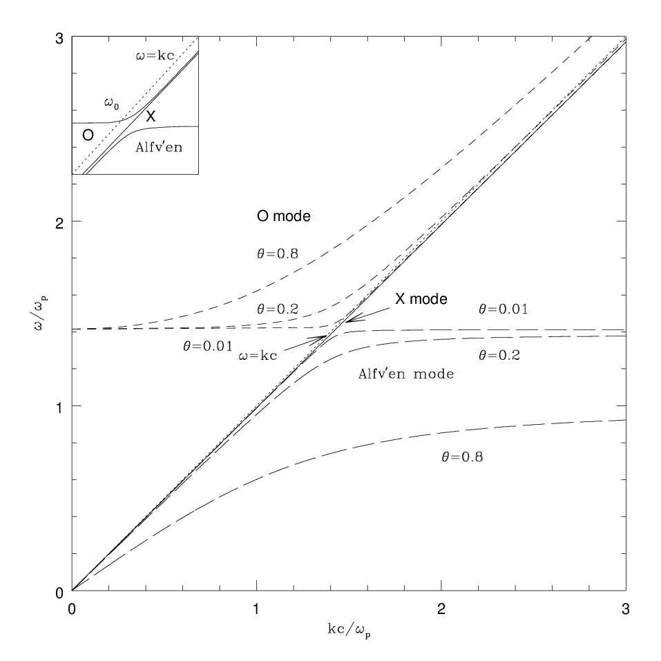
Equation (11) describes the transverse X wave with the electric vector perpendicular to the k-B plane and equation (12) describes the coupled longitudinal-transverse wave which has two branches: O quasi-transverse wave with the electric vector in the k-B plane and quasi-longitudinal Alfvén wave with the electric vector along B.

4.3 Parallel Propagation

The normal modes of the plasma for the parallel propagation are given by

	$\displaystyle\omega_{l}\,=\,\sqrt{2}\,\omega_{p}\mbox{}$		(13)
	$\displaystyle n_{t}^{2}=1+{2\,\omega_{p}^{2}\over\omega_{B}^{2}-\omega_{t}^{2}}$		(14)

(subscripts _l and _t refer to longitudinal and transverse polarizations of waves).

For exactly parallel propagation, the dispersion curves for the O mode and Alfvén mode intersect at

\omega^{\ast}=\sqrt{2}\omega_{p}\hskip 21.68121ptk^{\ast}c\approx\sqrt{2}\omega_{p}\left(1+\omega_{p}^{2}/{\omega_{B}}^{2}\right),\mbox{ for ${\omega_{p}\over\omega_{B}}\ll 1$ }

(15)

This intersection occurs only for the parallel propagation, while for oblique propagation the dispersion curves for O, X and Alfvén modes are well separated. It follows that equation (13) describes the O mode for $k\,<\,k^{\ast}$ and the Alfvén mode for $k\,>\,k^{\ast}$ , while equation (14) describes the X mode for all frequencies and the Alfvén mode for $k\,<\,k^{\ast}$ and the O mode for $k\,>\,k^{\ast}$ .

As the wave propagates in a curved magnetic field of the pulsar magnetosphere, it’s path on the CMA diagram (see Sections 4.6) depends on the branch that the wave belongs to. In the linear regime in wave amplitude and with the adiabatically changing parameters of a medium, a wave always stays on a given branch. For example, original electrostatic wave emitted along the magnetic field can acquire electromagnetic components as it propagates in the presence of a curved magnetic field. The linear evolution of the longitudinal plasma wave, emitted originally along the field line, will drastically depend on which branch (O or Alfvén) the wave actually belongs to. The propagation of O and Alfvén waves in the inhomogeneous plasma of a pulsar magnetosphere differs considerably (Arons & Barnard 1986, Barnard & Arons 1986). If the plasma wave is emitted with the wave vector (or frequency) above the intersection point $k\,>\,k^{\ast}$ , then the linear transformation of the longitudinal plasma wave will follow the Alfvén branch, which cannot escape magnetosphere. On the other hand, if the plasma wave is emitted with the wave vector below the intersection point $k\,<,k^{\ast}$ , then the linear transformation of the longitudinal plasma wave will follow the O branch, which may escape from plasma.

4.4 Oblique Propagation

In the pulsar magnetosphere the waves that may be important for the generation of the observed radio emission have frequencies much less than the gyrofrequency. In what follows, we will often use the low frequency approximation when all the relevant frequencies are much less than the gyrofrequency. In the cold plasma in its rest frame this implies: $\omega\ll\omega_{B}$ . The solution of equation (11) in the low frequency limit describes a subluminous transverse electromagnetic wave:

\omega^{2}=k^{2}c^{2}\left(1-{2\omega_{p}^{2}\over\omega_{B}^{2}}\right)=k^{2}v_{A}^{2},\hskip 14.45377pt\mbox{ $\omega\ll\omega_{B}$},\hskip 14.45377pt\mbox{ X mode}

(16)

where $v_{A}$ is the Alfvén velocity in a strongly magnetized plasma.

Solutions of equation (12) are more complicated. The simple form for the dispersion relation may be obtained near the cross-over point, where the dispersion relation of the O mode crosses the vacuum dispersion relation or in the asymptotic regimes far from the cross-over point.

Solving (12) with the refractive index set to unity we find the cross-over point for the O wave.

\omega_{0}^{2}=\,k_{0}^{2}\,c^{2}=\,2\,{{{\it\omega_{p}}}^{2}}+{{{\it{\omega_{B}}}}^{2}}\,{{\sin^{2}\theta}}

(17)

Near the cross-over point, the approximate dispersion relation for the O mode may be found using the relation

\omega-\omega_{0}=-\left.\left({\partial K(\omega,{\bf k})\over\partial{\bf k}}\right)\right/\left({\partial K(\omega,{\bf k})\over\partial\omega}\right)d{\bf k}

(18)

where $K(\omega,{\bf k})=0$ is the dispersion equation for $\omega({\bf k})$ .

From Eq. (12) we find

\omega=k_{0}\,c+\kappa(k-k_{0})c

(19)

where

	$\displaystyle\kappa={1\over c}\left.{\partial\omega\over\partial k}\right\|_{k=k_{0}}=\,{{{{{\it{\omega_{B}}}}^{4}}\,{{\cos^{2}\theta}}\,{{\sin^{2}\theta}}}\over{4\,{{{\it\omega_{p}}}^{4}}+2\,{{{\it{\omega_{B}}}}^{2}}\,{{{\it\omega_{p}}}^{2}}\,{{\sin^{2}\theta}}+{{{\it{\omega_{B}}}}^{4}}\,{{\cos^{2}\theta}}\,{{\sin^{2}\theta}}}}\mbox{}$
	$\displaystyle\,\approx\,1-{{4\,{{{\it\omega_{p}}}^{4}}}\over{4\,{{{\it\omega_{p}}}^{4}}+{{{\it{\omega_{B}}}}^{4}}\,{{\cos^{2}\theta}}\,{{\sin^{2}\theta}}}}$		(20)

where we used the assumption ${\omega_{B}}\,\gg\omega_{p}$ . From (20) it follows, that the behavior of the dispersion relation of the O wave near the cross-over point shows a very sensitive dependence on the angle of propagation. There exist a critical angle $\theta_{c}={2\omega_{p}^{2}/\omega_{B}^{2}}$ at which the dispersion relation changes:

		$\displaystyle\omega=\,\sqrt{2}\,\omega_{p}+{{\omega_{B}}^{4}\over 2\,\omega_{p}^{4}}\,(k-\,k_{0})c\,,\hskip 21.68121ptk_{0}^{2}\,\approx 2\,\omega_{p}^{2}/c^{2}$	if $\theta\,\ll 2\omega_{p}^{2}/{\omega_{B}}^{2}$		(21)
		$\displaystyle\omega=\,kc-{{{4\,\left(k-{\it k_{0}}\right)c\,{{{\it\omega_{p}}}^{4}}\,\over{{\sin^{2}\theta}}\,{{\cos^{2}\theta}}}{{{{\it{\omega_{B}}}}^{4}}}}},\hskip 7.22743ptk_{0}^{2}c^{2}\,=2\,\omega_{p}^{2}+\,{\omega_{B}}^{2}\,\sin^{2}\theta$	if $\theta\,\gg\,2\omega_{p}^{2}/{\omega_{B}}^{2}$		(21)

For angles smaller than $\theta_{c}$ we can generally use the approximation of parallel propagation when considering the dispersion relations of the waves, while for larger angles we must take into account the effects of oblique propagation.

The other limits when the dispersion relations for the O and Alfvén waves may be obtained in closed form are the asymptotic limits far from the cross-over point. The large and small wave vector asymptotic solutions are

	$\displaystyle\hskip-28.90755pt\omega^{2}=\left\{\begin{array}[]{ll}\phantom{{{{{a\over b}\over{a\over b}}}\over{{{a\over b}\over{a\over b}}}}}{k^{2}c^{2}}\,\left(1-{{2\,{{{\it\omega_{p}}}^{2}}\,{{\cos^{2}\theta}}}\over{{{{\it{\omega_{B}}}}^{2}}}}\right)+2\,{{{\it\omega_{p}}}^{2}}\,{{\sin^{2}\theta}}&\mbox{ O wave}\\ \phantom{{{{{a\over b}\over{a\over b}}}\over{{{a\over b}\over{a\over b}}}}}2\,{{{\it\omega_{p}}}^{2}}\,{{\cos^{2}\theta}}\,\left(1-{{2\,{{{\it\omega_{p}}}^{2}}\,{{\sin^{2}\theta}}}\over{{k^{2}c^{2}}}}-{{2\,{{{\it\omega_{p}}}^{2}}\,{{\sin^{2}\theta}}}\over{{{{\it{\omega_{B}}}}^{2}}}}\right)&\mbox{ Alfv\'{e}n wave}\end{array}\right.\hskip-21.68121pt\mbox{ if $kc\,\gg\omega_{p}$}\mbox{}$
	$\displaystyle\hskip-28.90755pt\omega^{2}=\left\{\begin{array}[]{ll}\phantom{{{{{a\over b}\over{a\over b}}}\over{{{a\over b}\over{a\over b}}}}}2\,{{{\it\omega_{p}}}^{2}}+{k^{2}c^{2}}\,\left(1-{{{k^{2}c^{2}}\,{{\cos^{2}\theta}}}\over{{{{\it\omega_{p}}}^{2}}}}\right)\,{{\sin^{2}\theta}}&\mbox{ O wave }\\ \phantom{{{{{a\over b}\over{a\over b}}}\over{{{a\over b}\over{a\over b}}}}}{k^{2}c^{2}}\,{{\cos^{2}\theta}}\,\left(1-{{2\,{{{\it\omega_{p}}}^{2}}}\over{{{{\it{\omega_{B}}}}^{2}}}}-{{{k^{2}c^{2}}\,{{\sin^{2}\theta}}}\over{2\,{{{\it\omega_{p}}}^{2}}}}\right)&\mbox{ Alfv\'{e}n wave}\end{array}\right.\hskip-14.45377pt\mbox{ if $kc\,\ll\omega_{p}$}$

4.5 Infinite Magnetic Field

In the limit of infinitely strong magnetic field the dispersion relations for the O (plus sign) and Alfvén modes (minus sign) are (Arons & Barnard 1986)

\omega^{2}={{k^{2}c^{2}}\over 2}+{{{\it\omega_{p}}}^{2}}\pm{{{\sqrt{{k^{4}}c^{4}+4\,{{{\it\omega_{p}}}^{4}}-4\,k^{2}\,c^{2}{{{\it\omega_{p}}}^{2}}\,\cos(2\,\theta)}}}\over 2}

(28)

The short and long wave length asymptotics are then given by (4.4) and (4.4) with the magnetic field set to infinity.

An important point in considering the wave excitation in the superstrong magnetic field is that we cannot neglect the very large but finite magnetic field. In the approximation of the infinitely strong magnetic field the O mode is always superluminous and thus cannot be excited by the Cherenkov-type resonant wave-particle interaction. In this limit any instability would occur on the Alfvén waves which are strongly damped as they propagate out in the pulsar magnetosphere. When the finite magnetic field is taken into account, O wave becomes subluminous for the small angles of propagation and can be resonantly excited by the Cherenkov, cyclotron or Cherenkov-drift interaction with the fast particles.

4.6 CMA Diagram for Cold Pair Plasma

CMA diagrams (e.g. Budden 1985) are useful tools in considering wave propagation. It is a plot of the refractive index versus some functions of wave, plasma and cyclotron frequencies. We chose the following coordinates for CMA diagram:

W={1\over Y^{2}}=\left({\omega\over\omega_{B}}\right)^{2},\hskip 14.45377ptZ={X\over Y^{2}}=\left({\omega_{p}\over\omega_{B}}\right)^{2}

(29)

where $Y$ and $X$ are the standard quantities in the magnetosonic theory. With this choice of coordinates the lines of constant $Z$ are the lines of constant density and are independent of wave frequency. The lines of constant $W$ are the lines of constant wave frequency and are independent of the density. The regions on the CMA diagram are separated by the resonance, where $n\rightarrow\infty$ , and cutoffs, where $n\rightarrow 0$ .

Using Eqs (11) and (12) we find resonance

		$\displaystyle W=1$	X modes		(30)
		$\displaystyle W={1\over 2}+Z\pm\sqrt{\left({1\over 2}+Z\right)^{2}-2Z\cos^{2}\theta}$	O & Alfvén modes		(31)

and reflection points

		$\displaystyle W=1+2Z$	X modes		(32)
		$\displaystyle\left\{\begin{array}[]{cc}W=1+2Z&\\ W=2Z\end{array}\right.$	O & Alfvén modes		(32)

For the $X$ wave the curve $n=1$ corresponds to $Z=0$ (vacuum case). For the O mode $n=1$ at $W=2Z+\sin^{2}\theta$ (cross-over point) and $Z=0$ (vacuum case). Other useful relations for the resonances of the coupled O and Alfvén modes are

		$\displaystyle{1\over 2}+Z+\sqrt{\left({1\over 2}+Z\right)^{2}-2Z\cos^{2}\theta}=$	$\displaystyle\left\{\begin{array}[]{cc}1&\mbox{ $\theta=0$}\\ 1+2Z&\mbox{ $\theta=\pi/2$}\\ 1+2Z\sin^{2}\theta&\mbox{ $Z\ll 1$}\\ 2Z+\sin^{2}\theta&\mbox{ $Z\gg 1$}\end{array}\right.\mbox{}$
		$\displaystyle{1\over 2}+Z-\sqrt{\left({1\over 2}+Z\right)^{2}-2Z\cos^{2}\theta}=$	$\displaystyle\left\{\begin{array}[]{cc}2Z&\mbox{ $\theta=0$}\\ 0&\mbox{ $\theta=\pi/2$}\\ 2Z\cos^{2}\theta&\mbox{ $Z\ll 1$}\\ \cos^{2}\theta&\mbox{ $Z\gg 1$}\end{array}\right.$

The CMA diagrams are plotted in Figs. 4 and 5.

4.7 Polarization of waves in cold plasma

To find the polarizations of the waves we construct a matrix of cofactors of $\Lambda$ (Melrose 1978) :

	$\displaystyle\lambda_{\alpha\beta}=n^{4}k_{\alpha}k_{\beta}-n^{2}\left(k_{\alpha}k_{\beta}\epsilon_{\gamma\gamma}+\delta_{\alpha\beta}k_{\gamma}k_{\eta}\epsilon_{\gamma\eta}-k_{\alpha}k_{\gamma}\epsilon_{\gamma\beta}-k_{\beta}k_{\gamma}\epsilon_{\alpha\gamma}\right)\mbox{}$
	$\displaystyle\hskip 21.68121pt+{1\over 2}\delta_{\alpha\beta}\left(\epsilon_{\gamma\gamma}^{2}-\epsilon_{\gamma\eta}\epsilon_{\eta\gamma}\right)+\epsilon_{\alpha\gamma}\epsilon_{\gamma\beta}-\epsilon_{\gamma\gamma}\epsilon_{\alpha\beta}$		(46)

Then the polarization vectors may be chosen as columns of $\lambda_{\alpha\beta}$ .

For cold plasma, the elements of $\lambda_{\alpha\beta}$ are

	$\displaystyle\lambda_{xx}=\left(-1+n^{2}-{\frac{2\,\omega_{p}^{2}}{-{{\omega}^{2}}+{{\omega_{B}}^{2}}}}\right)\,\left(-1+{\frac{2\,\omega_{p}^{2}}{{{\omega}^{2}}}}+n^{2}\,{{\sin^{2}\theta}}\right)\mbox{}$
	$\displaystyle\lambda_{xz}=n^{2}\,\left(-1+n^{2}+{\frac{2\,\omega_{p}^{2}}{{{\omega}^{2}}-{{\omega_{B}}^{2}}}}\right)\,\cos\theta\,\sin\theta=\lambda_{zx}\mbox{}$
	$\displaystyle\lambda_{yy}=-\left(\left(-1+n^{2}+{\frac{2\,\omega_{p}^{2}}{{{\omega}^{2}}}}\right)\,\left(1+{\frac{2\,\omega_{p}^{2}}{-{{\omega}^{2}}+{{\omega_{B}}^{2}}}}\right)\right)+{\frac{2\,n^{2}\,{{\omega_{B}}^{2}}\,\omega_{p}^{2}\,\cos^{2}\theta}{{{\omega}^{2}}\,\left(-{{\omega}^{2}}+{{\omega_{B}}^{2}}\right)}}\mbox{}$
	$\displaystyle\lambda_{zz}=\left(1-n^{2}+{\frac{2\,\omega_{p}^{2}}{-{{\omega}^{2}}+{{\omega_{B}}^{2}}}}\right)\,\left(1+{\frac{2\,\omega_{p}^{2}}{-{{\omega}^{2}}+{{\omega_{B}}^{2}}}}-n^{2}\,\cos^{2}\theta\right)$		(47)

We note that these relations are exact in frequency.

For the X mode using (11) for the refractive index in (47) we find the polarization vector for the X mode $e_{X}=(0,1,0)$ . For the O and Alfvén modes using (12) for the refractive index in (47) we obtain the ratio of the electric field components in the wave:

{E_{x}\over E_{z}}=-{\frac{\left({{\omega}^{2}}-{{\omega_{B}}^{2}}\right)\,\left({{\omega}^{2}}-2\,\omega_{p}^{2}\right)\,\cot\theta}{{{\omega}^{2}}\,\left({{\omega}^{2}}-{{\omega_{B}}^{2}}-2\,\omega_{p}^{2}\right)}}

(48)

For the point far from the cross-over point we can use the approximation of a very strong magnetic field to find

{E_{x}\over E_{z}}=\left(-1+{\frac{2\,\omega_{p}^{2}}{{{\omega}^{2}}}}\right)\,\left(1-2{\omega_{p}^{2}\over\omega_{B}^{2}}\right)\cot\theta

(49)

Using the relation (48) we can estimate the polarization of the O wave at the cross-over point. We find that

{E_{x}\over E_{z}}\approx{\frac{2\,{{\omega_{p}}^{2}}\,\theta}{{{\omega_{B}}^{2}}}}

(50)

For the angles smaller than ${\omega_{p}^{2}/\omega_{B}^{2}}$ the O wave is quasi-longitudinal at the cross-over point and for larger angles it is quasi-transverse.

Relations (49) and (50) allow us to find the normalized polarization vectors:

	$\displaystyle e_{O}=$		$\displaystyle\left\{\begin{array}[]{ll}\hskip-14.45377pt\phantom{{{{{a\over b}\over{a\over b}}}\over{{{a\over b}\over{a\over b}}}}}\left\{\cos\theta\,\left(1-{\frac{2\,{{\omega_{p}}^{2}}\,{{\sin^{2}\theta}}}{{{\omega}^{2}}}}\right),0,\left(1+{\frac{2\,{{\omega_{p}}^{2}}\,{{\cos^{2}\theta}}}{{{\omega}^{2}}}}\right)\,\sin\theta\right\}+O\left({\omega_{p}^{2}\over k^{2}c^{2}}\right)&\mbox{ $kc\,\gg\omega_{p}$}\\ \hskip-14.45377pt\phantom{{{{{a\over b}\over{a\over b}}}\over{{{a\over b}\over{a\over b}}}}}\left\{{\frac{-\left(k^{2}\,\sin(2\,\theta)\right)}{4\,\omega_{p}^{2}}},0,1\right\}+O\left({k^{2}c^{2}\over\omega_{p}^{2}}\right)&\mbox{ $kc\,\ll\omega_{p}$}\end{array}\right.\mbox{}$
	$\displaystyle\mbox{}e_{O}=$		$\displaystyle\left\{\begin{array}[]{ll}\phantom{{{{{a\over b}\over{a\over b}}}\over{{{a\over b}\over{a\over b}}}}}\left\{{\frac{{{\omega_{B}}^{2}}\,\theta}{{{\omega_{0}}^{2}}}},0,-1\right\}&\mbox{ $\theta\ll{2\omega_{p}^{2}\over\omega_{B}^{2}}$ }\\ \phantom{{{{{a\over b}\over{a\over b}}}\over{{{a\over b}\over{a\over b}}}}}\left\{1,0,-{\frac{{{\omega_{0}}^{2}}\,\csc\theta\,\sec\theta}{{{\omega_{B}}^{2}}}}\right\}&\mbox{ $\theta\gg{2\omega_{p}^{2}\over\omega_{B}^{2}}$}\end{array}\right.\hskip 14.45377pt\mbox{ $\omega\approx\omega_{0}$}\mbox{}$
	$\displaystyle\mbox{}e_{A}=$		$\displaystyle\left\{\begin{array}[]{ll}\hskip-14.45377pt\phantom{{{{{a\over b}\over{a\over b}}}\over{{{a\over b}\over{a\over b}}}}}\left\{\left(1+{\frac{2\,{{\omega_{p}}^{2}}\,{{\cos^{2}\theta}}}{k^{2}}}\right)\,\sin\theta,0,\cos\theta\,\left(1-{\frac{2\,{{\omega_{p}}^{2}}\,{{\sin^{2}\theta}}}{k^{2}}}\right)\right\}+O\left({\omega_{p}^{2}\over k^{2}}\right)&\mbox{ $kc\,\gg\omega_{p}$}\\ \hskip-14.45377pt\phantom{{{{{a\over b}\over{a\over b}}}\over{{{a\over b}\over{a\over b}}}}}\left\{1,0,{\frac{{{\omega}^{2}}\,\tan\theta}{2\,\omega_{p}^{2}}}\right\}+O\left({k^{2}c^{2}\over\omega_{p}^{2}}\right)&\mbox{ $kc\,\ll\omega_{p}$}\end{array}\right.$

which are accurate to $O\left({\omega_{p}^{2}\over{\omega_{b}}^{2}}\right)$ .

5 Waves in a Cold Pair Plasma in Pulsar Frame

In the pulsar magnetosphere the plasma is moving along the field lines with a bulk Lorenz factor $\gamma_{p}\approx 10-1000$ . In this frame the waves propagating in different directions have different dispersion relations. So that the dispersion equation for the X mode becomes a fourth order equation for $\omega({\bf k})$ . To simplify the consideration we will use the low frequency approximation from the very beginning, i.e. we expand all the relevant relations in $1/\omega_{B}$ . In what follows, the quantities measured in the pulsar frame will be denoted with primes.

For the forward propagating waves, which in the plasma frame has $\theta\ll 1$ , we obtain

	$\displaystyle\hskip-72.26999pt\omega_{X}^{\prime}=k^{\prime}c(1-\mbox{ {\large${\omega_{p}^{\prime\,2}\over 4\gamma_{p}^{3}\omega_{B}^{2}}$}})$
	$\displaystyle\omega_{O}^{\prime}=\left\{\begin{array}[]{ll}\phantom{{{{{a\over b}\over{a\over b}}}\over{{{a\over b}\over{a\over b}}}}}k^{\prime}c\left(1-\mbox{ {\large${\omega_{p}^{\prime\,2}\over 4\gamma_{p}^{2}\omega_{B}^{2}}+{\frac{\,\gamma_{p}{{\,\omega_{p}}^{\prime\,2}}\,{{\sin^{2}\theta^{\prime}}}}{{c^{2}}\,{k^{\prime\,2}}\,}}$}}\right)&\mbox{ if $k^{\prime}c\,\gg\,\gamma_{p}\omega_{p}^{\prime}$ }\\ \phantom{{{{{a\over b}\over{a\over b}}}\over{{{a\over b}\over{a\over b}}}}}v_{p}k^{\prime}+{\sqrt{2}\omega_{p}^{\prime}\over\gamma_{p}^{3/2}}&\mbox{ if $k^{\prime}c\,\ll\,\gamma_{p}\omega_{p}^{\prime}$ }\end{array}\right.\mbox{}$
	$\displaystyle\omega_{A}^{\prime}=\left\{\begin{array}[]{ll}\phantom{{{{{a\over b}\over{a\over b}}}\over{{{a\over b}\over{a\over b}}}}}k^{\prime}c\cos\theta^{\prime}\left(1-\mbox{ {\large${\,\omega_{p}^{\prime\,2}\,\over 4\,\gamma_{p}^{3}\,\omega_{B}^{2}}\,-{\frac{{c^{2}}\,{k^{\prime\,2}}\,{{\sin^{2}\theta^{\prime}}}}{4\,\gamma_{p}{{\,\omega_{p}}^{\prime\,2}}}}$}}\right)&\mbox{ if $k^{\prime}c\,\ll\,\gamma_{p}\omega_{p}^{\prime}$ }\\ \phantom{{{{{a\over b}\over{a\over b}}}\over{{{a\over b}\over{a\over b}}}}}v_{p}k^{\prime}+\mbox{ {\large${\sqrt{2}\omega_{p}^{\prime}\cos\theta^{\prime}\over\gamma_{p}^{3/2}}$}}&\mbox{ if $k^{\prime}c\,\gg\,\gamma_{p}\omega_{p}^{\prime}$ }\end{array}\right.$

The plasma frequencies in the two frames are related by $\omega_{p}^{\prime}=\omega_{p}/\sqrt{\gamma_{p}}$ .

The cross-over point, where the O mode becomes luminal, is

\omega_{0}^{\prime\,2}={2\omega_{p}^{\prime\,2}\over\gamma_{p}}+{4\gamma_{p}^{2}\omega_{B}^{2}\theta^{\prime\,2}}

(66)

6 Waves in a Relativistically Hot Pair Plasma

6.1 Effects of Thermal Motion on Wave Dispersion

In this section we consider wave propagation in the relativistically hot, strongly magnetized electron-positron plasma. The thermal motion of plasma particles affects considerably the dispersion of the Alfvén mode at frequencies $\omega\geq\omega_{p}$ and the dispersion of the O mode frequencies $\omega\approx\omega_{p}$ . Another important quantitative modification is in the dispersion relation of the X mode. An important factor for the excitation of the X mode is the difference of its phase speed and the speed of light. This difference is roughly proportional to $<1/\gamma^{3}>$ (Eq. 87). It is decreased considerably by the bulk streaming of the plasma. In the relativistically hot streaming plasma there are more particles with low Lorentz factors, that contribute to $<1/\gamma^{3}>$ , than in the cold plasma streaming with with the same average velocity. So for a given streaming velocity relativistically hot plasma has larger $<1/\gamma^{3}>$ and larger growth rate.

6.2 Distribution functions

To estimate the thermal effects on the dispersion of the plasma mode we use the two kinds of distribution functions: (i) waterbag distribution

f(p_{z})=\,\left\{\begin{array}[]{ll}{n_{p}\over 2p_{T}},&\mbox{ if $-p_{T}\,<p_{z}\,<p_{T}$}\\ 0,&\mbox{ otherwise}\end{array}\right.

(67)

(here $p_{T}\approx mc\gamma_{T}$ is the scatter in moments) and (ii) relativistic Maxwellian distribution (see also Appendices B and C for the calculations of the relevant moments of the distribution)

f(p_{z})={n_{p}\over 2K_{1}(\beta_{T})}\exp\left\{-\beta_{T}p_{\mu}U^{\mu}\right\}

(68)

here $\beta_{T}=1/T_{p}$ , $T_{p}$ is the invariant temperature, $p_{\mu}$ is a four-momentum of the particle, $U^{\mu}$ is four velocity of the reference frame, $K_{1}$ is a modified Bessel function. In most of the calculations to follow we will assume that the plasma is very hot: $p_{T}/mc\gg 1$ and $\,T_{p}=\sqrt{p_{T}^{2}/(mc)^{2}+1}\gg 1$ .

Both these distributions are ”fast falling” at large moments. This is an important factor for the dispersion relation of plasma waves (see below). The advantage of the water bag distribution is that the various moments of the distribution can be easily calculated. The relativistic Maxwellian distribution is explicitly Lorentz-invariant (see Appendix B for details of Lorentz transformation).

The relevant moments of the distributions are summarized in Table 1 for the water bag distribution (in the plasma frame only) and in Table 2 for the relativistic Maxwellian distribution (in both plasma and pulsar frame).

$<\gamma>$	$<pv>$	$<{1\over\gamma}>$	$<{1\over\gamma^{3}}>$
$\gamma_{T}/2$	$\gamma_{T}/2$	${\ln\gamma_{T}\over\gamma_{T}}$	${1\over\gamma_{T}}$

Table 1: Relevant moments of the water bag distribution in its rest frame (dimensionless units). It is assumed that

p_{T}/m_{e}c\approx\gamma_{T}\gg 1

[Uncaptioned image] — Table 2: Moments of the one-dimensional relativistic Maxwellian distribution

The water bag distribution is generally a good approximation for the account of the thermal motion of the particles. Its major drawback is the absence of a tail of high energy particles, that can resonate with the waves in the plasma. The Cherenkov resonance on the tail particles will result in a strong damping of the waves. The cyclotron resonance on the tail particles may result in a wave excitation if the distribution function is asymmetric with a long high energy tail. The condition, that the Cherenkov resonance is unimportant, is that the phase speed of the waves in plasma is much larger, than the thermal velocity of the particles. In the case of the idealized water bag distribution this condition has to be put in by hand. Whenever the phase speed of the wave becomes comparable to the thermal velocity the waves should be considered strongly damped and nonexistent. Therefore, we expect that the high frequency branch of the Alfvén wave, which in the limit of cold plasma had a very low phase velocity, will be strongly damped.

Here, we should also mention a long standing controversy about the dispersion of the longitudinal waves and the possibility of the two stream instabilities in the relativistic plasma. In the initial work (Silin 1960) and later works (Suvorov & Chugunov 1975) it was stated that the relativistic plasma does not support subluminous longitudinal waves. This problem has been considered anew (Tsytovich & Kaplan 1972) who found subluminous waves. The controversy has been resolved by Lominadze & Mikhailovskii 1978 who demonstrated the existence of the subluminous waves in the range $0<n-1<1/<\gamma>^{2}$ ( $n\approx 1$ ), provided that the third moment of the distribution ( $<\gamma^{3}>$ ) is finite (here $n$ is the refractive index and $<\gamma>\gg 1$ is the average Lorentz factor of the plasma particles). Thus, when the distribution function falls off at large momenta slower than $1\over\gamma^{4}$ subluminous plasma waves do not exist.

For the water bag distribution, the dispersion of the plasma waves for the parallel propagation is given by Eq. (72). We find that $n-1$ becomes larger than $1/\,T_{p}^{2}$ for $\omega>\mbox{ several times }\omega_{0}$ . For larger frequencies the Longitudinal plasma waves are either strongly damped or do not exist at all (Silin 1960).

6.3 Dispersion Relations in Relativistic Pair Plasma

To simplify the analysis we will use the low frequency approximation $\omega\,\ll{\omega_{B}}$ and the assumption of a very strong magnetic field ${\,T_{p}\omega_{p}^{2}\over{\omega_{B}}^{2}}\,\ll 1$ from the very beginning. The dielectric tensor is then given by

$\displaystyle\epsilon_{xx}$	$\displaystyle=1+d\,\,T_{p}\,\left(1+n^{2}\,\beta_{T}^{2}\,\cos^{2}\theta\right)\,\,=\epsilon_{yy}\mbox{}$
$\displaystyle\mbox{}\epsilon_{zz}$	$\displaystyle=1-{\frac{2\,n^{2}\,\omega_{p}^{2}}{\,T_{p}\,\left(1-n^{2}\,\beta_{T}^{2}\,\cos^{2}\theta\right)}}+d\,\,T_{p}\,n^{2}\,{{\sin^{2}\theta}}\mbox{}$
$\displaystyle\mbox{}\epsilon_{xy}$	$\displaystyle=\epsilon_{yx}=\epsilon_{xz}=\epsilon_{zx}=\epsilon_{yz}=\epsilon_{zy}$	(69)

where

d={\omega_{p}^{2}\over\omega_{B}^{2}},\hskip 21.68121pt\beta_{T}=\sqrt{1-{1\over T_{p}^{2}}}

(70)

The normal modes of a hot plasma are given by the solution of (9) with the dielectric tensor (69). Similarly to the cold case, equation (69) factorizes into a dispersion relation for the X mode and a coupled equation for the Alfvé and O modes.

6.4 Parallel Propagation

In the case of parallel propagation the dispersion equation gives two transverse wave with the dispersion

\omega^{2}=k^{2}\,c^{2}\left(1-d\,\,T_{p}(1+\beta_{T}^{2})\right)

(71)

and a plasma wave

\omega^{2}={2\,\omega_{p}^{2}\over\,T_{p}}+k^{2}c^{2}\beta_{T}^{2}

(72)

It is also useful to represent the dispersion relations for the plasma waves near the cross-over point in the form (19). For the relativistic plasma components we find

	$\displaystyle\left.\left({\partial K(\omega,k)\over\partial k}\right)\right/\left({\partial K(\omega,k)\over\partial\omega}\right)=\left(1-{<\gamma(1+v)^{2}>\over<\gamma^{3}(1+v)^{3}>}\right)\mbox{}$
	$\displaystyle\omega\approx kc-{1\over T^{2}}(k-k_{0})$		(73)

The phase speed for the high frequency asymptotic of the plasma wave (72) approaches the phase speed of the thermal particles $c\beta_{T}$ . For the more realistic distribution function, these parts of the dispersion relation will be strongly damped on the Cherenkov resonance with the thermal tail particles. The high frequency asymptotic of the plasma wave belongs to the Alfvén wave. From this we make a conclusion that the high frequency ( $kc\geq\,T_{p}\omega_{p}$ ) part of the Alfvén wave is strongly damped and does not propagate.

6.5 Oblique Propagation

The dispersion relation for the X mode is

\omega^{2}=\,k^{2}c^{2}\left(1-\,d\,T_{p}\,\left(1+\beta_{T}^{2}\,\cos^{2}\theta\right)\right)

(74)

The dispersion relations for the O and Alfvén waves in a hot pair plasma are plotted in Fig. 6.

It is possible to obtain the asymptotic expansion of the dispersion relation of Alfvén and O modes in the limits of very small and very large wave vectors. In the limit $kc\,\gg\sqrt{\,T_{p}}\omega_{p}$ we have

\omega^{2}\,=\,\left\{\begin{array}[]{ll}\hskip-14.45377pt\phantom{{{{{a\over b}\over{a\over b}}}\over{{{a\over b}\over{a\over b}}}}}{c^{2}}\,k^{2}\,\beta_{T}^{2}\,\cos^{2}\theta\,\left(1-\mbox{{\large${\frac{2\,\omega_{p}^{2}}{{c^{2}}\,{\,T_{p}^{3}}\,k^{2}\,\beta_{T}^{2}\,\left(-1+\beta_{T}^{2}\,\cos^{2}\theta\right)}}$}}\right)&\hskip-14.45377pt\mbox{ Alfv\'{e}n wave}\\ \hskip-14.45377pt\phantom{{{{{a\over b}\over{a\over b}}}\over{{{a\over b}\over{a\over b}}}}}{c^{2}}\,k^{2}\,\left(1-d\,\,T_{p}\,\left(1+\beta_{T}^{2}\,\cos^{2}\theta\right)\right)\,\left(1-\mbox{{\large${\frac{2\,\omega_{p}^{2}\,{{\sin^{2}\theta}}}{{c^{2}}\,\,T_{p}\,k^{2}\,\left(-1+\beta_{T}^{2}\,\cos^{2}\theta\right)}}$}}\right)&\mbox{ O-wave}\end{array}\right.

(75)

while in the opposite limit $kc\,\ll\,\sqrt{\,T_{p}}\omega_{p}$

\omega^{2}\,=\,\left\{\begin{array}[]{ll}\phantom{{{{{a\over b}\over{a\over b}}}\over{{{a\over b}\over{a\over b}}}}}{c^{2}}\,k^{2}\,\cos^{2}\theta\,\left(1-d\,\,T_{p}\,\left(1+\beta_{T}^{2}\,\cos^{2}\theta\right)\right)\,\left(1-{\frac{{c^{2}}\,k^{2}\,{{\sin^{2}\theta}}}{2\,\,T_{p}\,\omega_{p}^{2}}}\right)&\mbox{ Alfv\'{e}n wave}\\ \phantom{{{{{a\over b}\over{a\over b}}}\over{{{a\over b}\over{a\over b}}}}}\frac{2\,\omega_{p}^{2}}{\,T_{p}}+{c^{2}}\,k^{2}\,\left(\beta_{T}^{2}\,\cos^{2}\theta+{{\sin^{2}\theta}}\right)&\mbox{ O-wave}\end{array}\right.

(76)

The X mode is always superluminous and the Alfvén mode is always subluminous. The O mode is superluminous for small small vectors $kc\,\ll\sqrt{T_{p}}\omega_{p}$ and may become subluminous for very small angles of propagation $\theta\ll\sqrt{T_{p}}\omega_{p}/\omega_{B}$ .

The cross-over point (where the phase speed of the O mode become equal to the speed of light) is now $\omega_{0}^{2}\,=k_{0}^{2}c^{2}\,\approx\,2\,\,T_{p}\omega_{p}^{2}+{{\omega_{B}}^{2}\sin^{2}\theta}$ . Using relation (18) we can approximate the dispersion relation near the cross-over point as

\omega=kc-\kappa(k-k_{0}),\hskip 14.45377pt\kappa={1\over T^{2}}-{(\omega_{B}^{4}+4T_{p}^{3}\omega_{B}^{2}\omega_{p}^{2})\theta^{2}\over 16T_{p}^{6}\omega_{p}^{4}}

(77)

6.6 Polarization of waves in a hot plasma

In the case of a hot plasma the matrix of cofactors $\lambda^{(h)}_{\alpha\beta}$ is quite complicated and is not given here. Simple relations may be obtained in the limit $\omega_{B}=\infty$ and near the cross-over point for the O wave. In the limit $\omega_{B}=\infty$ we find the elements of the matrix $\lambda^{(h)}_{\alpha\beta}$

	$\displaystyle\lambda^{(h)}_{xx}=\left(-1+n^{2}\right)\,\left(-1-{\frac{2\,\omega_{p}^{2}}{\,T_{p}\,{{\omega}^{2}}\,\left(-1+n^{2}\,v_{0}^{2}\,\cos^{2}\theta\right)}}+n^{2}\,{{\sin^{2}\theta}}\right)\mbox{}$
	$\displaystyle\lambda^{(h)}_{xz}=n^{2}\,\left(-1+n^{2}\right)\,\cos\theta\,\sin\theta=\lambda^{(h)}_{zx}\mbox{}$
	$\displaystyle\lambda^{(h)}_{yy}=1-n^{2}-{\frac{2\,\omega_{p}^{2}\,\left(-1+n^{2}\,\cos^{2}\theta\right)}{\,T_{p}\,{{\omega}^{2}}\,\left(-1+n^{2}\,v_{0}^{2}\,\cos^{2}\theta\right)}}\mbox{}$
	$\displaystyle\lambda^{(h)}_{zz}=\left(-1+n^{2}\right)\,\left(-1+n^{2}\,\cos^{2}\theta\right)$		(78)

For the X mode we find that the polarization vector is $e_{X}=(0,1,0)$ , while for the O mode

{E_{x}\over E_{z}}={\frac{n^{2}\,\cos\theta\,\sin\theta}{-1+n^{2}\,\cos^{2}\theta}}

(79)

These relations are valid for the points not close to the cross-over point of the O wave (near the cross-over point the approximation $\omega_{B}=\infty$ is not applicable). Near the cross-over point, $n=1$ , we find

{E_{x}\over E_{z}}=-{\frac{{{\omega_{B}}^{2}}\theta}{{4T_{p}^{3}{\omega_{p}}^{2}}}}

(80)

For oblique propagation the behavior of the O mode at the cross-over point changes at

\theta\approx{4T_{p}^{3}d}

(81)

For smaller angles the O mode is quasiparallel at the cross-over point while, for large angles, it is quasitransverse.

The polarization vectors for the O and Alfvén modes are then given by

	$\displaystyle e_{O}^{(h)}=\left\{\begin{array}[]{ll}\left\{\cos\theta\,\left(1-{\frac{2\,T_{p}\,\omega_{p}^{2}\,{{\sin^{2}\theta}}}{c^{2}k^{2}}}\right),0,-\left(\left(1+{\frac{2\,T_{p}\,\omega_{p}^{2}\,\cos^{2}\theta}{c^{2}k^{2}}}\right)\,\sin\theta\right)\right\},&\mbox{ $kc\,\gg\omega_{p}$}\\ \left\{{\frac{{{\omega_{B}}^{2}}\,\theta}{{{\omega_{0}}^{2}}}},0,-1\right\}&\hskip-144.54pt\mbox{ $\theta\ll{2\,T_{p}\omega_{p}^{2}\over\omega_{B}^{2}},\,\,$ $\omega=\omega_{0}^{(h)}$ }\\ \left\{1,0,-{\frac{{{\omega_{0}}^{2}}}{{{\sin\theta\cos\theta\omega_{B}}^{2}}}}\right\}&\hskip-144.54pt\mbox{ $\theta\gg{2\,T_{p}\omega_{p}^{2}\over\omega_{B}^{2}},\,\,$ $\omega=\omega_{0}^{(h)}$ }\end{array}\right.\mbox{}$
	$\displaystyle e_{A}^{(h)}=\left\{1,0,{\frac{{{\omega}^{2}}\,\tan\theta}{2\,\,T_{p}\,\omega_{p}^{2}}}\right\}\hskip 72.26999pt\mbox{ $kc\,\ll\omega_{p}$}$		(86)

6.7 Dispersion Relation for Hot Pair Plasma in Pulsar Frame

The dispersion relations for the forward propagating modes in the pulsar frame in the limit $\,\omega^{\prime}\ll\,\omega_{B}$ are

	$\displaystyle\omega^{\prime}_{X}\,=\,k^{\prime}c\left(1-{\,\omega_{p}^{\prime\,2}T_{p}\over 4\,\omega_{B}^{2}\,\gamma_{p}^{3}}\right)$
$\displaystyle\mbox{}\hat{\omega}_{O}\,=\,$	$\displaystyle k^{\prime}c\left(1-{\,\omega_{p}^{\prime\,2}\,T_{p}\,\over 4\,\gamma_{p}^{3}\,\omega_{B}^{2}}\,+{\frac{\gamma_{p}{{\,\omega_{p}}^{\prime\,2}}T_{p}\,{{\sin^{2}\theta^{\prime}}}}{{c^{2}}\,{k^{2}}\,}}\right)$	if $k^{\prime}c\,\gg\sqrt{T_{p}}\,\gamma_{p}\omega_{p}^{\prime}$ and $\theta^{\prime}<1/T_{p}$
$\displaystyle\mbox{}\hat{\omega}_{A}\,=\,$	$\displaystyle k^{\prime}c\cos\theta^{\prime}\left(1-{\,\omega_{p}^{\prime\,2}\,T_{p}\,\over 2\,\gamma_{p}^{3}\,\omega_{B}^{2}}\,-{\frac{{c^{2}}\,{k^{\prime\,2}}\,{{\sin^{2}\theta^{\prime}}}}{2\,T_{p}\,\,\gamma_{p}{{\,\omega_{p}}^{\prime\,2}}}}\right)$	if $kc\,\ll\,\sqrt{T_{p}}\,\gamma_{p}\omega_{p}$	(87)

These relationships are valid for the frequencies satisfying the inequality

\,\omega\ll\,\gamma_{p}\,\omega_{B}/T_{p}

(88)

This is a condition that in the reference frame of the plasma the frequency of the waves is much smaller that the typical cyclotron frequency of the particles $\,\omega_{B}/T_{p}$ .

The cross-over point in this frame is

\omega_{0}^{\prime\,2}={2\omega_{p}^{\prime\,2}T_{p}\over\gamma_{p}}+{4\gamma_{p}^{2}\omega_{B}^{2}\theta^{\prime\,2}}

(89)

7 Hydrodynamic and Kinetic Instabilities

The description of the beam-plasma instabilities is based on the scheme used to solve the general problem of linear oscillations in plasma. The initial equations are the linearized kinetic equations for the particles in a self-consistent electromagnetic field and Maxwell’s equations. When the unperturbed state of the beam and plasma is stationary and spatially uniform, we can use Eq. (9) to find the normal modes of a medium.

For the beam-plasma system the dielectric tensor $\epsilon_{\alpha\beta}(\omega,{\bf k})$ may be represented as a sum of contributions from plasma and beam.

\epsilon_{\alpha\beta}(\omega,{\bf k})=\delta_{\alpha\beta}+{4\pi c\over\omega}\sigma_{\alpha\beta}^{plasma}+{4\pi c\over\omega}\sigma_{\alpha\beta}^{beam}

(90)

where $\sigma_{\alpha\beta}^{plasma}$ and $\sigma_{\alpha\beta}^{beam}$ are the conductivity tensors of plasma and beam.

Sometimes it is possible to consider beam as a weak perturbation to the system. Then, in the zeroth approximation, the normal modes of the medium will be determined from (9) with $\sigma_{\alpha\beta}^{beam}$ set to zero. This will produce a set of normal modes of the medium $\left\{\omega({\bf k})^{l}\right\}$ .

If the plasma alone is stable, then the frequency of the normal modes will have a zero imaginary part. In the first approximation, dispersion relation (9) may be expanded taking into account a small contribution to the dielectric tensor from the beam. The frequency shift $\Delta({\bf k})^{l}$ of the normal mode $\omega({\bf k})^{l}$ is then determined from

\Delta({\bf k})^{l}\left.\left[{\partial\over\partial\omega}K_{p}(\omega,{\bf k})\right]\right|_{\omega({\bf k})^{l}}+K_{b}(\omega,{\bf k})=0

(91)

where $K_{p}(\omega,{\bf k})$ and $K_{b}(\omega,{\bf k})$ are the plasma and beam parts of Eq.(9). For stable plasma without a beam, $K_{p}(\omega,{\bf k})$ and $\left\{\omega({\bf k})^{l}\right\}$ are real.

Two separate cases may be distinguished here depending on whether the complex part of the beam contribution to the dispersion relations (91) $K_{b}(\omega,{\bf k})$ is zero or nonzero. If Im( $K_{b}(\omega,{\bf k})=0$ then equation (91) has real coefficients. The complex solutions of Eq.(91) (if any) are complex conjugates. Solutions with the positive complex part correspond to the growing waves. These are hydrodynamic instabilities. In hydrodynamic instabilities, all the particles of the beam resonate with the normal mode of the plasma. This requires that the growth rate of the instability be greater than the intrinsic bandwidth of the growing waves:

|{\bf k\cdot\delta v}|\ll{\rm Im}(\Delta({\bf k})).

(92)

Here ${\bf k}$ is the resonant wave vector, ${\bf\delta v}$ is the scatter in the velocity of the beam particles. This is satisfied for a very small scatter in the velocity of the beam particles, so that all the particles from the beam resonate with the beam.

Alternatively, if the complex part of the the beam contribution to the dispersion relations (91) $K_{b}(\omega,{\bf k})$ is nonzero, the frequency shift $\Delta({\bf k})$ will always have a complex part. If the complex part of $\Delta({\bf k})^{l}$ is larger than zero, then the corresponding normal mode $\omega({\bf k})^{l}$ will be growing at the expense of the beam energy, while for negative $\Delta({\bf k})^{l}$ the mode will be damped on the resonant particles of the beam. This case corresponds to the kinetic instability. The requirement that the frequency shift $\Delta({\bf k})^{l}$ due to the complex part of $K_{b}(\omega,{\bf k})$ dominates over the shift due to the large real part of $K_{b}(\omega,{\bf k})$ requires that the growth rate be much less than the the intrinsic bandwidth of the growing waves (reversed inequality (92)). This is satisfied for a very large scatter in the velocity of the beam particles, so that at any given moment only a small fraction of the beam particles is in resonance with the wave.

Though the physical interpretations of the kinetic and hydrodynamic instabilities are quite different, they may be considered as two limiting cases of a general beam instability. For a relativistic beam traveling along a magnetic field with average Lorentz factor $\gamma_{b}$ , scatter in parallel Lorentz factors $\Delta\gamma$ , and average pitch angle $\psi$ the condition of the hydrodynamic approximation (92) takes the form

k_{\parallel}c\,\left({\psi^{2}\over 2}+{\Delta\gamma\over\gamma^{3}}\right)\,+k_{\perp}c\,\psi+{s\omega_{B}\Delta\gamma\over\gamma^{2}}\,\ll\Gamma

(93)

where $s$ is the harmonic number ( $s=0$ for Cherenkov resonance, $s\neq 0$ for cyclotron resonance) and $\Gamma$ is a growth rate of an instability. For the kinetic instability, this inequality is reversed.

From (93) it follows that there exist a critical pitch angle

\psi_{crit}={1\over\gamma}\,\sqrt{{\Delta\gamma\over\gamma}}

(94)

For $\psi>\psi_{crit}$ the scatter in pitch angles dominates over longitudinal velocity spread. For $\psi>\psi_{crit}$ the average ”longitudinal” mass of the beam particles decreases by the factor of $(\psi\gamma_{b})^{2}$ so that the instabilities whose growth rate is inversely proportional to the ”longitudinal” mass of the particles (like Cherenkov instability of plasma waves) may be enhanced considerably.

Relativistic particles propagating along the curved magnetic field of a pulsar magnetosphere initially are in the ground quantum state (zero pitch angle). They can develop a finite pitch angle by (i) particle-particle collisions, (ii) interaction with the electromagnetic field (Compton scattering on the diffuse thermal photons or recoil due the emission of electromagnetic waves at anomalous cyclotron resonance), and (iii) when the adiabatic approximation for the propagation breaks down (when the Larmor radius becomes comparable with the size of the inhomogeneity). The pitch angle of the particles is then determined by the balance of these forces on one hand and radiation damping at the normal synchrotron resonance and the force due to the conservation of adiabatic invariant on the other hand.

In magnetosphere, the particle-particle collision time is very long compared with the dynamical time because of the relatively low density of particles, high speed and the one-dimensional character of the motion. We also assume that the Compton scattering on the diffuse thermal photons is unimportant and that the adiabatic approximation for the propagation of particles is satisfied. The transverse component of the force due to the radiation damping at normal synchrotron resonance dominates the transverse motion of the particles near the neutron star, making the pitch angles equal to zero. Then the pitch angles will remain zero throughout the region where the above conditions are satisfied.

In what follows we assume that plasma is one-dimensional before the development of instabilities. The condition of hydrodynamic approximation (93) is then

k_{\parallel}c\,{\Delta\gamma\over\gamma^{3}}+{s\omega_{B}\Delta\gamma\over\gamma^{2}}\,\ll\Gamma

(95)

In the kinetic regime this inequality is reversed.

For an instability to be important as a possible source of coherent emission generation, its growth rate, evaluated in the pulsar frame, should be much larger than the pulsar rotation frequency $\Omega$ . The growth rates in the pulsar and plasma frames are related by

\Gamma^{\prime}={\Gamma\over\gamma_{p}}.

(96)

So the requirement of a fast growth in the plasma frame is

{\Gamma\over\gamma_{p}\Omega}\gg 1.

(97)

Another, more stringent requirement on the growth rate comes from the angular dependence of a growth rate. The emitting plasma propagates in a curved magnetic field. If an instability has a considerable growth inside a characteristic angle $\delta\theta^{\prime}$ , then the growth length should be larger than $\delta\theta R_{c}$ , where $R_{c}$ is the curvature of the magnetic fields. In the plasma frame this requirement is

\Gamma\gg{c\gamma_{p}^{2}\over R_{c}\,\delta\theta},

(98)

where we used $\delta\theta^{\prime}\approx\delta\theta/\gamma_{p}$ .

8 Cold Pair Plasma: Resonances

In the cold plasma approach the resonant interaction between the fast particles and the plasma may be considered as the interaction of the waves in the plasma with the waves in the beam. The interaction is the strongest when the dispersion relations of the waves intersect. Consequently, we are looking for the possible resonances between the waves in the plasma (12) and the waves in the beam (see Fig. 7 and 8):

	$\displaystyle\omega=v_{b}\,k_{z}\mbox{}$		(99)
	$\displaystyle\omega=v_{b}\,k\cos\theta\pm{\omega_{B}\over\gamma_{b}}$		(100)

As we will see in Section 10, the resonant interaction of the plasma waves with the Cherenkov waves in the beam (99) is described by the cubic equation for the frequency shift, which always has complex conjugate solutions. This implies that the Cherenkov resonant interaction of the waves in the beam and in the plasma is always unstable.

In contrast, the frequency shift due to the cyclotron interaction of the waves in the beam and in the plasma (100) is described by a quadratic equation, which has two real solutions for the plus sign in (100) and two complex solutions for the minus sign in (100). Thus, only the minus sign in (100) will contribute to the instability growth rate. The resonance (100) with the minus sign is called anomalous Doppler resonance. This corresponding instability may be considered as the interaction of the negative energy wave in the beam with the positive energy wave in plasma. Due to the resonant coupling, the amplitudes of both waves grow exponentially.

Now let us consider the condition for the resonances (99) and (100) to occur. From the low frequency asymptotics of the Alfvén waves (4.4) we infer that the possibility of the Cherenkov excitation of the Alfvén waves depends on the parameter

\mu\,=\,{2\,\gamma_{b}\,\omega_{p}\over{\omega_{B}}}

(101)

If $\mu\,<\,1$ , then Alfvén waves can be excited by Cherenkov resonance.¹¹ 1 In the case of cold plasma this may be considered as a sufficient condition for the Cherenkov excitation of Alfvén waves. In the case of hot plasma this is only a necessary condition (see below). However, if $\mu\,>\,1$ then Alfvén waves cannot be excited by Cherenkov resonance. Instead, resonance can occur for an O mode subject to the requirement of sufficiently small angles of propagation Fig. 8.

For the cold plasma in the region of open field lines we have

\mu\,=\,\gamma_{b}\sqrt{{2\,\lambda\,\Omega\over\gamma_{p}{\omega_{B}}}}=\,\sqrt{{2\,\lambda\,\Omega\over{\omega_{B}}}}{\gamma_{b}^{\prime}\over\gamma_{p}^{3/2}}\,=\,5\times 10^{-3}\left({r\over R_{NS}}\right)^{3/2}\,=\,\left\{\begin{array}[]{ll}<1,&\mbox{ if $\left({r\over R_{NS}}\right)<43$}\\ >1,&\mbox{ if $\left({r\over R_{NS}}\right)>43$}\end{array}\right.

(102)

So, at small radii ( $\mu\ll 1$ ) it is the Alfvén wave that is excited by the Cherenkov resonance, while for larger radii ( $\mu\geq 1$ ) it is the O-mode that can be excited by the Cherenkov resonance. In the outer parts of magnetosphere ( $r\geq 100R_{NS}$ ) the parameter $\mu$ becomes much larger than unity: $\mu\gg 1$ .

For the parallel propagation (and only in this case) the parts of the O and Alfvén modes that have longitudinal polarization may be considered as forming a single plasma wave with a dispersion $\omega\,=\,\sqrt{2}\omega_{p}$ . In this particular case, the excitation of either O or Alfvén part of the longitudinal plasma mode is very similar. But as the waves propagate in the curved magnetic field lines, the parts of the plasma mode corresponding to the O or Alfvén wave will evolve differently resulting in a different observational characteristics of the emergent radiation.

In what follows we consider separately the two possible cases of Cherenkov resonances: $\mu>1$ and $\mu<1$ .

We also note that the X wave cannot be excited by the Cherenkov resonance. Though the formal intersection of the Cherenkov wave in the beam (99) with the dispersion relation of the X mode is possible for all frequencies if $\mu=1$ , the transverse polarization of the X mode excludes a resonant interaction with particles streaming along the magnetic field.

The cyclotron resonance on the X modes occurs at $\omega_{\rm res}\,\,\ll{\omega_{B}}$ , provided that

{\omega_{p}^{2}\gamma_{b}\over{\omega_{B}}^{2}}\gg 1

(103)

Using the fiducial plasma parameters of the cold plasma, we find

{\omega_{p}^{2}\gamma_{b}\over{\omega_{B}}^{2}}\,=\,\lambda\,\gamma_{b}{2\Omega\over\gamma_{p}{\omega_{B}}}={\lambda\gamma_{b}^{\prime}\over\gamma_{p}^{2}}{\Omega\over{\omega_{B}}}\,=\,1.3\times 10^{-10}\left({r\over R_{NS}}\right)^{3}

(104)

which implies that the X mode can be excited by the cyclotron resonance only in the outer parts of magnetosphere for radii satisfying

\left({r_{\rm res}\,\over R_{NS}}\right)\,>\left({\omega_{B}^{\ast}\gamma_{p}^{2}\over\lambda\gamma_{b}^{\prime}\Omega}\right)^{1/3}\approx 2\times 10^{3}\,

(105)

The location of the cyclotron resonance on the X mode is quite sensitive to the choice of the bulk streaming energy. Comparing the resonant frequency (Table 3) with the plasma frequency, we find

{\omega_{\rm res,X,cycl}\over\omega_{p}}\,=\,{{\omega_{B}}^{3}\over\gamma_{b}\,\omega_{p}^{3}}\,=\,{\gamma_{p}^{3/2}\over\gamma_{b}\lambda^{3/2}}\left({\omega_{B}\over 2\Omega}\right)^{3/2}\,\gg 1

(106)

which implies that the X mode is always excited with the frequencies much larger than the plasma frequency.

Locations of the resonances in the cold plasma are given in Table 3.

9 Hydrodynamic Instabilities In Cold Plasma

9.1 Dielectric Tensor for Cold Beam-Plasma System

The dielectric tensor for beam of the density $n_{b}$ propagating with the velocity $v_{b}$ along the magnetic field $B$ through a plasma of the density $n$ can be found from a general expression (Eq 5) with zero drift velocity $u_{\alpha}=0$ and distribution function $f_{\alpha}(p_{z})=n_{p}\,\delta(p_{z})+n_{b}\delta(p_{z}-p_{b})$ ( $n_{b}$ is a density of a beam and $p_{z}$ is a momentum of beam particles):

$\displaystyle\epsilon_{xx}$	$\displaystyle=1+{{2\,{{{\it\omega_{p}}}^{2}}}\over{-{{\omega}^{2}}+{{{\it{\omega_{B}}}}^{2}}}}-{{{{{\it{\omega_{b}}}}^{2}}\,{{{\it\hat{\omega}}}^{2}}}\over{{\it\gamma_{b}}\,{{\omega}^{2}}\,{{{\it\tilde{{\omega}}}}^{2}}}}\,=\epsilon_{yy}\mbox{}$
$\displaystyle\mbox{}\epsilon_{xy}$	$\displaystyle={{-i\,{{{\it{\omega_{b}}}}^{2}}\,{\it{\omega_{B}}}\,{\it\hat{\omega}}}\over{{{{\it\gamma_{b}}}^{2}}\,{{\omega}^{2}}\,{{{\it\tilde{{\omega}}}}^{2}}}}=-\epsilon_{yx}\mbox{}$
$\displaystyle\mbox{}\epsilon_{xz}$	$\displaystyle=-{{k\,{{{\it{\omega_{b}}}}^{2}}\,{\it\hat{\omega}}\,{\it v_{b}}\,\sin\theta}\over{{\it\gamma_{b}}\,{{\omega}^{2}}\,{{{\it\tilde{{\omega}}}}^{2}}}}=\epsilon_{zx}\mbox{}$
$\displaystyle\mbox{}\epsilon_{yz}$	$\displaystyle={{i\,k\,{{{\it{\omega_{b}}}}^{2}}\,{\it{\omega_{B}}}\,{\it v_{b}}\,\sin\theta}\over{{{{\it\gamma_{b}}}^{2}}\,{{\omega}^{2}}\,{{{\it\tilde{{\omega}}}}^{2}}}}=-\epsilon_{zy}\mbox{}$
$\displaystyle\mbox{}\epsilon_{zz}$	$\displaystyle=1-{{2\,{{{\it\omega_{p}}}^{2}}}\over{{{\omega}^{2}}}}-{{{{{\it{\omega_{b}}}}^{2}}}\over{{{{\it\gamma_{b}}}^{3}}\,{{{\it\hat{\omega}}}^{2}}}}-{{k^{2}\,{{{\it{\omega_{b}}}}^{2}}\,{{{\it v_{b}}}^{2}}\,{{\sin^{2}\theta}}}\over{{\it\gamma_{b}}\,{{\omega}^{2}}\,{{{\it\tilde{{\omega}}}}^{2}}}}$	(107)

where $\hat{\omega}\,=\,\omega-\,k\,v_{b}\,\cos\theta$ , $\tilde{{\omega}}^{2}\,=\,(\omega-\,k\,v_{b}\,\cos\theta)^{2}-{\omega_{B}}^{2}/\gamma_{b}^{2}$ and $\gamma_{b}=1/\sqrt{1-{v_{b}^{2}\over c^{2}}}$ .

We will always assume that beam can be considered as a weak perturbation, so that we can employ the expansion procedure described in Section 7.

9.2 Parallel Propagation

In this section we calculate the growth rates for the beam instabilities for the waves propagating along the magnetic field, that we will use later as guide lines for the general case of oblique propagation.

For the propagation along the magnetic field the dispersion relation (9) with a dielectric tensor 107 factorizes:

	$\displaystyle-1+{2\,\omega_{p}^{2}\over\omega^{2}}+{\omega_{b}^{2}\over\gamma_{b}^{3}\,\hat{\omega}^{2}}=0\mbox{}$		(108)
	$\displaystyle-1+n^{2}+{{2\,{{{\it\omega_{p}}}^{2}}}\over{{\omega^{2}}-{{{\it{\omega_{B}}}}^{2}}}}+{{{{{\it{\omega_{b}}}}^{2}}\,{\it\hat{\omega}}}\over{{\it\gamma_{b}}\,{\omega^{2}}\,\left(\pm\,{{{\it{\omega_{B}}}}/{{\it\gamma_{b}}}}+{\it\hat{\omega}}\right)}}=0$		(109)

Equation (108) describes hydrodynamic excitation of longitudinal plasma waves. As discussed above, this may be a longitudinal part of Alfvén or O mode depending on the parameters of plasma.

Equation (109) describes the cyclotron excitation of the O and X modes. For the parallel propagation the cyclotron excitation of the Alfvén wave does not occur.

9.3 Cherenkov Excitation of Plasma Waves for $\theta=0$

We now look for the correction to the relations (13) and (99) when the two intersect.

	$\displaystyle\omega\,=$		$\displaystyle\,\sqrt{2}\omega_{p}+\Delta\mbox{}$
	$\displaystyle\mbox{}\omega\,=$		$\displaystyle v_{b}\,k\cos\theta+\Delta$		(110)

Expanding in small $\Delta$ , we find that the frequency shift satisfies a third order equation:

-{\frac{{\sqrt{2}}\,{{\Delta}^{3}}}{\omega_{p}}}+{\frac{{{\omega_{b}}^{2}}}{{{\gamma_{b}}^{3}}}}=0

(111)

Equation (111) always has one real and two complex conjugated roots. The complex root with the positive complex part corresponds to the instability.

Solving Eq. (111), we find the complex part of the frequency shift:

{\rm Im}(\ \Delta)={{{\sqrt{3}}\,{{{\it\omega_{p}}}^{{1\over 3}}}\,{{{\it{\omega_{b}}}}^{{2\over 3}}}}\over{{2^{{7\over 6}}}\,{\it\gamma_{b}}}}={\sqrt{3}\lambda^{1/6}\sqrt{\Omega{\omega_{B}}}\over 2^{2/3}\gamma_{b}\sqrt{\gamma_{p}}}

(112)

This is a growth rate for the Cherenkov excitation of plasma waves (c.f. Godfrey et al. 1975, Egorenkov et al. 1983).

We can compare the importance of the Cherenkov excitation of plasma waves by evaluating growth rate (112) for the set of fiducial parameters of a cold plasma and comparing it with the dynamical time (96):

{{\rm Im}(\ \Delta)\over\gamma_{p}\Omega}\approx{\lambda^{1/6}\over\gamma_{b}\gamma_{p}^{3/2}}\sqrt{{\omega_{B}}\over\Omega}=86\left({y\over R_{NS}}\right)^{-3/2}

(113)

From which it follows that this instability may be important for $r\,\leq 20$ . We will see in Section 10 that the second criterion (98) is not satisfied for the Cherenkov excitation of Alfvén or O waves, so that the Cherenkov instability does not develop.

9.4 Cyclotron Excitation of Transverse Waves for $\theta=0$

We expect that the hydrodynamic instability will be strongest at small wave vectors. We can then use the low frequency approximation (16) to the dispersion of the transverse waves. We seek the correction to the relations (16) and (100) when the two intersect.

	$\displaystyle\omega\,=$		$\displaystyle\,kc\,\left(1-{\omega_{p}^{2}\over{\omega_{B}}^{2}}\right)+\ \Delta\mbox{}$
	$\displaystyle\mbox{}\omega\,=$		$\displaystyle\,k\,v_{b}\,\cos\theta-{{\omega_{B}}\over\gamma_{b}}+\ \Delta$		(114)

Expanding in small $\Delta$ , we find that the frequency shift satisfies the quadratic equation:

-{\frac{\Delta\,k^{2}c^{2}}{{{\omega}^{3}}}}\pm{\frac{\omega_{B}\,{{\omega_{b}}^{2}}}{\Delta\,\gamma_{b}\,{{\omega}^{2}}}}=0

(115)

The $\pm$ sign in (115) corresponds to the two signs in (109). For the normal Doppler resonance (plus sign in (109) and (115)) the resulting frequency shift is real. For the anomalous Doppler resonance, the frequency shift is complex:

\Delta\,=\,\pm{{i\,{\sqrt{\omega}}\,{\sqrt{{\it{\omega_{B}}}}}\,{\it{\omega_{b}}}}\over 2{{\it\gamma_{b}}\,kc}}

(116)

which gives near the resonant frequency (Table 3)

{\rm Im}(\Delta)=\,{{i\,{\it\omega_{p}}\,{\it{\omega_{b}}}}\over 2\,{{\sqrt{{\it\gamma_{b}}}}\,{\it{\omega_{B}}}}}={\sqrt{\lambda}\Omega\over\gamma_{p}\sqrt{\gamma}_{b}}

(117)

For the parameters of a cold plasma the growth rate (117) is much longer than the dynamical time everywhere inside the light cylinder.

{{\rm Im}(\ \Delta)\over\gamma_{p}\Omega}\approx{\sqrt{\lambda}\over\gamma_{p}^{2}\sqrt{\gamma_{b}}}=10^{-4}\ll 1

(118)

Which implies that hydrodynamic regime of the cyclotron instability is unimportant.

9.5 Perpendicular Propagation

Next, we consider the hydrodynamic instabilities for the waves propagating perpendicular to the magnetic field (magnetized Wiebel instability (Weibel 1959)). The normal modes of plasma without a beam for $\theta=\,\pi/2$ follow from Eq. (9):

	$\displaystyle{{\omega}^{2}}=k^{2}+2\,{{{\it\omega_{p}}}^{2}}\mbox{}$		(119)
	$\displaystyle{{\omega}^{2}}={{{\it{\omega_{B}}}}^{2}}+2\,{{{\it\omega_{p}}}^{2}}\mbox{}$		(120)
	$\displaystyle n^{2}=1+{{2\,{{{\it\omega_{p}}}^{2}}}\over{-{{\omega}^{2}}+{{{\it{\omega_{B}}}}^{2}}}}$		(121)

In the limit ${\omega_{B}}\,\rightarrow\,\infty$ the two solution of the biquadratic Eq. (121) may be expanded in large ${\omega_{B}}$ :

	$\displaystyle{{\omega}^{2}}={{{\it{\omega_{B}}}}^{2}}+2\,{{{\it\omega_{p}}}^{2}}+{{2\,{c^{2}}\,k^{2}\,{{{\it\omega_{p}}}^{2}}}\over{{{{\it{\omega_{B}}}}^{2}}}}\mbox{}$		(122)
	$\displaystyle{{\omega}^{2}}={c^{2}}\,k^{2}\,\left(1-{{2\,{{{\it\omega_{p}}}^{2}}}\over{{{{\it{\omega_{B}}}}^{2}}}}\right)$		(123)

In the limit $kc\ll{\omega_{B}}$ the dispersion curves (122) and (120) approach each other near the upper hybrid frequency: ${{\omega}^{2}}={{{\it{\omega_{B}}}}^{2}}+2\,{{{\it\omega_{p}}}^{2}}$ . We then expand determinant (107) for $\theta=\pi/2$ near the upper hybrid frequency $\omega=\sqrt{{\omega_{B}}^{2}+2\,\omega_{p}^{2}}+\ \Delta$ keeping the terms up to the second order in $\ \Delta$ .

-{\frac{{{\Delta}^{2}}\,{{\omega_{B}}^{2}}}{{\omega_{p}^{4}}}}+{\frac{{c^{2}}\,\Delta\,k^{2}}{{\omega_{B}}\,\omega_{p}^{2}}}-{\frac{{c^{2}}\,k^{2}\,{\omega_{b}}^{2}}{\gamma_{b}\,{{\omega_{B}}^{4}}}}=0

(124)

Solving Eq. (124), we find the frequency shift

\ \Delta={{k\,{{{\it\omega_{p}}}^{2}}\,\left({\sqrt{{\it\gamma_{b}}}}\,k-{\sqrt{{\it\gamma_{b}}\,k^{2}-4\,{{{\it{\omega_{b}}}}^{2}}}}\right)}\over{2\,{\sqrt{{\it\gamma_{b}}}}\,{{{\it{\omega_{B}}}}^{3}}}}

(125)

which shows an instability for $kc\,<\,{{2\,{\it{\omega_{b}}}}/{{\it\gamma_{b}}}}$ with a maximum growth rate

{\rm Im}(\ \Delta)_{max}\approx\,{{{{{\it\omega_{p}}}^{2}}\,{{{\it{\omega_{b}}}}^{2}}}\over{{{{\it\gamma_{b}}}^{{3\over 2}}}\,{{{\it{\omega_{B}}}}^{3}}}}

(126)

which is negligible for all reasonable pulsar plasma parameters.

10 Oblique Wave Excitation in Cold Plasma in the Hydrodynamic Regime

In this section we develop a general theory of the hydrodynamic weak beam instabilities in the cold magnetized electron-positron plasma. We expand (107) in small ${\omega_{b}}$ keeping only first terms. After considerable algebra we obtain

	$\displaystyle\left(1-n^{2}+{{2\,{{{\it\omega_{p}}}^{2}}}\over{-{{\omega}^{2}}+{{{\it{\omega_{B}}}}^{2}}}}\right)\,\left(\left(-1+n^{2}+{{2\,{{{\it\omega_{p}}}^{2}}}\over{{{\omega}^{2}}}}\right)\,\left(1-{{2\,{{{\it\omega_{p}}}^{2}}}\over{{{\omega}^{2}}-{{{\it{\omega_{B}}}}^{2}}}}\right)\right.\mbox{}$
	$\displaystyle\left.\hskip 144.54pt+{{2\,n^{2}\,{{{\it{\omega_{B}}}}^{2}}\,{{{\it\omega_{p}}}^{2}}\,{{\cos^{2}\theta}}}\over{{{\omega}^{2}}\,\left({{\omega}^{2}}-{{{\it{\omega_{B}}}}^{2}}\right)}}\right)+\mbox{}$
	$\displaystyle{{\omega_{b}}^{2}\over\gamma_{b}^{3}\,\hat{\omega^{2}}}\left(-1+n^{2}\cos^{2}\theta+{2\,\omega_{p}^{2}\over\omega^{2}-{\omega_{B}}^{2}}\right)\,\left(-1+n^{2}+{2\,\omega_{p}^{2}\over\omega^{2}-{\omega_{B}}^{2}}\right)+\mbox{}$
	$\displaystyle{{{{{\it{\omega_{b}}}}^{2}}}\over\gamma_{b}{{{{\it\tilde{{\omega}}^{2}}}}}}\left({{2\,kc\,n^{2}\,\left(-1+n^{2}+{{2\,{{{\it\omega_{p}}}^{2}}}\over{{{\omega}^{2}}-{{{\it{\omega_{B}}}}^{2}}}}\right)\,{\it\hat{\omega}}\,{\it\beta_{b}}\,\cos\theta\,{{\sin^{2}\theta}}}\over{\,{{\omega}^{2}}}}+\right.\mbox{}$
	$\displaystyle{{k^{2}c^{2}\,\left(-1+n^{2}\right)\,{{{\it\beta_{b}}}^{2}}\,\left(-1+n^{2}\,{{\cos^{2}\theta}}\right)\,{{\sin^{2}\theta}}}\over{\,{{\omega}^{2}}}}+\mbox{}$
	$\displaystyle{2\,k^{2}c^{2}\,{{{\it\omega_{p}}}^{2}}\,{{{\it\beta_{b}}}^{2}}\,\left({{2\,\left(-{{\omega}^{2}}+{{{\it{\omega_{B}}}}^{2}}+{{{\it\omega_{p}}}^{2}}\right)}\over{{{\omega}^{2}}\,{{\left(-{{\omega}^{2}}+{{{\it{\omega_{B}}}}^{2}}\right)}^{2}}}}+{{n^{2}\,\left(1+{{\cos^{2}\theta}}\right)}\over{{{\omega}^{2}}\,\left({{\omega}^{2}}-{{{\it{\omega_{B}}}}^{2}}\right)}}\right)\,{{\sin^{2}\theta}}}+\mbox{}$
	$\displaystyle\left.{\hat{\omega}^{2}\over\omega^{2}}\left(\phantom{{{{{a\over b}\over{a\over b}}}\over{{{a\over b}\over{a\over b}}}}}\left(-1+{2\,\omega_{p}^{2}\over\omega^{2}}\right)\,\left(-2+n^{2}+{{4\,{{{\it\omega_{p}}}^{2}}}\over{{{\omega}^{2}}-{{{\it{\omega_{B}}}}^{2}}}}+n^{2}\,{{\cos^{2}\theta}}\right)\right.\right.\mbox{}$
	$\displaystyle\left.\left.\phantom{{{{{a\over b}\over{a\over b}}}\over{{{a\over b}\over{a\over b}}}}}+n^{2}\,\left(-2+n^{2}+{4\,\omega_{p}^{2}\over\omega^{2}-\omega_{B}^{2}}\right)\,\sin^{2}\theta\right)\right)$		(127)

The term containing $1/\hat{\omega^{2}}$ contribute to Cherenkov excitation and the term containing $1/\tilde{{\omega}}^{2}$ contribute to the cyclotron excitation.

To find the growth rates we expand the plasma part of (127) near the plasma modes (Eqs. (11) and (12)) and the beam part near the resonances $\hat{\omega}\,=\,0$ (for Cherenkov excitation) or $\tilde{\omega}\,=\,0$ (for cyclotron instability). The expansion of the plasma part of (127) near the plasma modes is done according to the relation

\omega\,=\,\omega^{(0)}+\Delta\left({\partial K_{p}\over\partial\omega}\right)\left|{}_{\omega^{(0)}}\phantom{{a\over b}}\right.

(128)

where $K_{p}$ is the plasma part of the determinant (107)

	$\displaystyle K_{p}\,=\,\left(1-n^{2}+{{2\,{{{\it\omega_{p}}}^{2}}}\over{-{{\omega}^{2}}+{{{\it{\omega_{B}}}}^{2}}}}\right)\mbox{}$
	$\displaystyle\times\,\left(\left(-1+n^{2}+{{2\,{{{\it\omega_{p}}}^{2}}}\over{{{\omega}^{2}}}}\right)\,\left(1-{{2\,{{{\it\omega_{p}}}^{2}}}\over{{{\omega}^{2}}-{{{\it{\omega_{B}}}}^{2}}}}\right)+{{2\,n^{2}\,{{{\it{\omega_{B}}}}^{2}}\,{{{\it\omega_{p}}}^{2}}\,{{\cos^{2}\theta}}}\over{{{\omega}^{2}}\,\left({{\omega}^{2}}-{{{\it{\omega_{B}}}}^{2}}\right)}}\right)$		(129)

and $\omega^{(0)}$ are the solutions of the equation $K_{p}=0$ .

Simultaneously, in the beam part of the Eq. (127) we should use the normal modes of the medium for the estimates of $\omega$ and the refractive index $n$ .

10.1 Excitation of Alfvén waves

We recall that the Cherenkov excitation of Alfvén waves is possible only for $\mu<1$ (Section 8). Expanding in small $\Delta$ near the Alfvén wave dispersion relation in the limit of infinite magnetic field and using the resonant frequency (Table 3) we can find the growth rate

\Delta=\left\{\begin{array}[]{ll}\phantom{{{{{a\over b}\over{a\over b}}}\over{{{a\over b}\over{a\over b}}}}}{\frac{{\sqrt{3}}\,{\omega_{p}^{{\frac{1}{3}}}}\,{{\omega_{b}}^{{\frac{2}{3}}}}\,{{\cos\theta}^{{\frac{1}{3}}}}}{{2^{{\frac{7}{6}}}}\,\gamma_{b}}}&\mbox{ if $\theta\,\ll\,1/\gamma_{b}$}\\ \phantom{{{{{a\over b}\over{a\over b}}}\over{{{a\over b}\over{a\over b}}}}}{\frac{{\sqrt{3}}\,{\omega_{p}^{{\frac{1}{3}}}}\,{{\omega_{b}}^{{\frac{2}{3}}}}\,\cot\theta}{{2^{{\frac{7}{6}}}}\,{\gamma_{b}^{{\frac{8}{3}}}}}}&\mbox{ if $\theta\,\gg\,1/\gamma_{b}$}\end{array}\right.

(130)

The hydrodynamic growth rate of the Alfvén waves has a maximum for parallel propagation. The numerical estimate of the maximum rate for Cherenkov excitation of Alfvén wave is given by (113) subject to the condition $\mu<1$ ( Section 8).

We can now compare the instability growth length with the coherence length (98). Using the estimate $\delta\theta\sim 1/\gamma_{b}$ we have

{R_{c}\delta\theta{\rm Im}\Delta\over c\gamma_{p}^{2}}\approx{R_{c}\Omega\over c}{\lambda^{1/6}\over\gamma_{p}^{3}\gamma_{b}^{2}}\sqrt{{\omega_{B}\over\Omega}}\ll 1

(131)

which implies that the Cherenkov instability on the Alfvén waves is unimportant.

10.1.1 Cyclotron excitation of Alfvén waves

Near the cyclotron resonance $\tilde{\omega}=0$ we keep in (127) only the terms proportional to $1/\tilde{\omega}^{2}$ . We consider two separate case depending on whether $\mu$ is larger or smaller than unity.

For $\mu<1$ (i.e. near the neutron star surface) using the short wave length asymptotics of the Alfvén branch (4.4) and the resonance condition (100) we find a pair of complex solutions

\Delta\,=\,\pm i{\frac{{\sqrt{\omega}_{p}}\,{\omega_{b}}\,{\sqrt{\cos\theta}}\,\sin\theta}{{2^{{\frac{5}{4}}}}\,{\sqrt{\omega_{B}}}}}=\,{\lambda^{1/4}\Omega{\sqrt{\cos\theta}}\,\sin\theta\over\sqrt{2}\gamma_{p}^{3/4}}\left({{\omega_{B}}\over\Omega}\right)^{1/4}

(132)

This frequency shift agrees with the $\delta_{-}^{C3}$ of the Table 3, region 3 of Godfrey Godfrey et al. 1975.

The ratio of the growth rate in equation (132) to the dynamical time is

{{\rm Im}(\Delta)\over\Omega\gamma_{p}}={\gamma_{b}^{1/4}{\sqrt{\cos\theta}}\,\sin\theta\over\sqrt{2}\gamma_{p}^{2}}\left({{\omega_{B}}\over\Omega}\right)^{1/4}\leq 150\left({r\over R_{NS}}\right)^{-3/4}

(133)

The criteria of a short growth length (97) gives

{R_{c}\delta\theta{\rm Im}(\Delta)\over c\gamma_{p}^{2}}\approx{R_{c}\Omega\over c}{\lambda^{1/4}\over\gamma_{p}^{11/4}}\left({{\omega_{B}}\over\Omega}\right)^{1/4}=1.6\left({r\over R_{NS}}\right)^{-3/4}

(134)

where we have approximated the trigonometric functions by unity.

The equations (133) and (134) imply that the cyclotron excitation of Alfvén wave in the hydrodynamic regime may be marginally important near the neutron star (see also Sections 13.1.2 and Eq. 158).

For $\mu\gg 1$ and $\theta\gg 1/\sqrt{\mu}$ (this case corresponds to the resonant frequency much smaller than $\omega_{p}$ ) using the short wave length asymptotics of the Alfvén branch (4.4) and the resonance condition (100) we find a pair of complex solutions

\Delta=\pm i{\frac{{{\omega_{B}}^{{\frac{1}{3}}}}\,{\omega_{b}}\,{{\tan\theta}^{{\frac{1}{3}}}}}{{2^{{\frac{5}{6}}}}\,{\gamma_{b}^{{\frac{5}{6}}}}\,{\omega_{p}^{{\frac{1}{3}}}}}}=\pm i{\Omega\tan^{1/3}\theta\over 2^{3/2}\lambda^{1/6}\gamma_{b}^{5/6}\gamma_{p}^{1/3}}\left({{\omega_{B}}\over\Omega}\right)^{2/3}

(135)

Comparing this growth rate with the dynamical time we obtain

{{\rm Im}(\Delta)\over\Omega\gamma_{p}}={\tan\theta^{1/3}\over 2^{3/2}\lambda^{1/6}\gamma_{b}^{5/6}\gamma_{p}^{4/3}}\left({{\omega_{B}}\over\Omega}\right)^{2/3}\approx 3\times 10^{4}\tan\theta^{1/3}\left({r\over R_{NS}}\right)^{-2}

(136)

where we estimated the typical angle of emission by unity. The ratio (136) is larger than unity for $r/R_{NS}\geq 43$ .

The second criteria on the growth rate (98) becomes

{R_{c}\delta\theta{\rm Im}(\Delta)\over c\gamma_{p}^{2}}\approx{R_{c}\Omega\over c}{1\over\lambda^{1/6}\gamma_{b}^{5/6}\gamma_{p}^{7/3}}\left({\omega_{B}\over\Omega}\right)^{2/3}=120\left({r\over R_{NS}}\right)^{-2}

(137)

which implies that the cyclotron excitation of Alfvén waves is efficient in the region where $\mu>1$ ( ${r\over R_{NS}}\geq 43$ ).

10.2 Excitation of the X wave

Using (127) we see that X mode is not emitted by the Cherenkov resonance since the corresponding term is zero if evaluated at the X mode (11).

Near the cyclotron resonance we obtain for the X mode a pair of complex solutions

{\it\Delta}=\pm{i\over 2}\,{\sqrt{{\omega_{B}}}\,{\it{\omega_{b}}}\over\gamma_{b}\,\sqrt{\omega}}

(138)

where we used $kc\,\approx\omega$ . Using Table 3 we obtain a growth rate for the cyclotron excitation of the X mode

{\it\Delta}=\pm{{{i}\,{\it\omega_{p}}\,{\it{\omega_{b}}}}\over 2\,{{\sqrt{{\it\gamma_{b}}}}\,{\it{\omega_{B}}}}}

(139)

The growth rate is almost constant inside the cone $\theta<{2\omega_{p}\over{\omega_{B}}}$ and is zero for larger $\theta$ . The growth rate (139) was also obtained for the case of parallel propagation (117). As we saw in Section 9.2 the hydrodynamic instability on the X mode is unimportant.

10.3 Excitation of the O mode

10.3.1 Cherenkov resonance ( $\mu>1$ )

Starting with (127) we expand the plasma part near the dispersion relation for O mode (12) and the beam part near Cherenkov resonance (99) $n=1/(\beta_{b}\cos\theta)$ . In the low frequency approximation $\omega\ll\omega_{B}$ O wave can be excited by Cherenkov resonance only if $\mu>1$ . We distinguish two cases: $\mu\geq 1$ and $\mu\gg 1$ . In the former case the resonance occurs at approximately cross-over point for the O wave while in the latter case the resonance occurs at $\omega\gg\omega_{0}$ .

In the case $\mu\geq 1$ with $\omega_{\rm res}\,$ given in Table 3, the growth rate is

\Delta={\frac{{\sqrt{6}}\,{{\omega_{B}}^{{\frac{2}{3}}}}\,\omega_{p}\,{{\omega_{b}}^{{\frac{2}{3}}}}\,\sin\theta}{2\,{{\gamma_{b}}^{{\frac{2}{3}}}}\,{{\left(-1+{{\mu}^{2}}\right)}^{{\frac{1}{6}}}}\,{{\left(8\,{{\omega_{p}}^{4}}+2\,{{\omega_{B}}^{2}}\,{{\sin^{2}\theta}}\right)}^{{\frac{1}{3}}}}}}

(140)

The growth rate is proportional to the angle of propagation with respect to the magnetic field. This is due to the increase of the potential part of the O mode with the angle. The case of $\mu=1$ corresponds to the unlikely case when the beam velocity is exactly equal to the Alfvén velocity. The growth rate (140) is valid for $\theta<1/\gamma_{b}$ . For all practical purposes this growth rate is very small.

In the case $\mu\gg 1$ the complex shifts of the frequencies near the Cherenkov resonance $\hat{\omega}=\Delta$ are given by

	$\displaystyle{\rm Im}(\Delta)\,=\,$		$\displaystyle{\frac{{\sqrt{3}}\,{\omega_{p}^{{\frac{2}{3}}}}\,{{\omega_{b}}^{{\frac{2}{3}}}}\,{\sqrt{2\,\omega_{p}^{2}+{{\omega_{B}}^{2}}\,{{\sin^{2}\theta}}}}}{2\,\gamma_{b}\,{{\left(4\,{\omega_{p}^{4}}+{{\omega_{B}}^{4}}\,{{\sin^{2}\theta}}\right)}^{{\frac{1}{3}}}}}}\,=\mbox{}$
			$\displaystyle\left\{\begin{array}[]{ll}\phantom{{{{{a\over b}\over{a\over b}}}\over{{{a\over b}\over{a\over b}}}}}{\sqrt{3}{\omega_{b}}^{2/3}\,\omega_{p}^{1/3}\over 2^{7/6}\gamma_{b}}&\mbox{ if $\theta\,\ll\,{2\omega_{p}^{2}\over{\omega_{B}}^{2}}$}\\ \phantom{{{{{a\over b}\over{a\over b}}}\over{{{a\over b}\over{a\over b}}}}}\sqrt{{3\over 2}}\,{\omega_{p}^{5/3}\,{\omega_{b}}^{2/3}\over\gamma_{b}{\omega_{B}}^{4/3}\sin^{2/3}\theta}&\mbox{ if $\theta\,\gg\,{2\omega_{p}^{2}\over{\omega_{B}}^{2}}$}\end{array}\right.\mu\gg 1$

The maximum growth rate is reached for the parallel propagation, while for oblique propagation the growth rate falls off as $\theta^{-2/3}$ . We have already estimated the growth rate for the parallel propagation (113) and found that it can be marginally efficient. We can apply the second requirement on the growth rate which relates the characteristic angle of emission and the radius of curvature (98). Estimating $\delta\theta\approx{\omega_{p}^{2}\over{\omega_{B}}^{2}}$ we find

{R_{c}\delta\theta{\rm Im}\Delta\over c\gamma_{p}^{2}}=\left({\lambda^{4/3}\over\gamma_{p}^{3}}\right)\left({\Omega\over{\omega_{B}}}\right)\left({R_{c}\Omega\over c}\right)\ll 1

(144)

which implies that the Cherenkov instability on the O mode does not develop.

10.3.2 Cyclotron excitation of the O mode

The growth rate for the cyclotron excitation of the O mode in the hydrodynamic regime may be estimated from the growth rate for the cyclotron excitation of the X mode (138) with the resonant frequency given in Table 3. The maximum growth rate is reached for the parallel propagation and is equal to the cyclotron growth rate of the X mode (138). The growth rate (138) decreases with the increase of the resonant frequency. Since the cyclotron resonance on the O mode happens at the frequencies larger than the the cyclotron resonance on the X mode, the corresponding growth rate of the O mode are smaller for oblique propagation.

We conclude this section by the table of the hydrodynamic growth rate in a cold plasma (Table 4).

11 Relativistic Pair Plasma: Resonances

From the low frequency approximation to the Alfvén waves dispersion we find that the possibility of Cherenkov excitation of Alfvén wave in a relativistic hot plasma depends on the parameter

\mu_{h}=\sqrt{{2\gamma_{b}^{2}\,T_{p}\omega_{p}^{2}(1+\beta_{T}^{2})\over{\omega_{B}}^{2}}}\approx{2\gamma_{b}\sqrt{\,T_{p}}\omega_{p}\over{\omega_{B}}}

(145)

(compare with (101)).

Using our fiducial numbers parameter $\mu$ may be estimated

\mu_{h}=2\gamma_{b}\sqrt{{\,T_{p}\lambda\Omega\over\omega_{B}\gamma_{p}}}==5\times 10^{-3}\left({r\over R_{NS}}\right)^{3/2}\,=\,\left\{\begin{array}[]{ll}<1,&\mbox{ if $\left({r\over R_{NS}}\right)<43$}\\ >1,&\mbox{ if $\left({r\over R_{NS}}\right)>43$}\end{array}\right.

(146)

Numerically $\mu_{h}$ and $\mu$ are equal for the chosen set of the fiducial numbers for the cold and hot cases.

Similarly to the cold case, the parameter $\mu_{h}$ determines the possibility of the excitation of the Alfvén and O waves. If $\mu_{h}\,<\,1$ then the O wave cannot be excited by Cherenkov resonance. In this case the Alfvén wave may be excited by the Cherenkov interaction subject to the condition that the resonance occurs on the parts of the dispersion curve that are not strongly damped (see below). If $\mu_{h}\,>\,1$ then the O wave may excited by Cherenkov resonance for the angles of propagation $\theta<{\sqrt{\,T_{p}}\omega_{p}\over{\omega_{B}}}$ .

Another limitation on the possible resonance comes from the requirement that the waves in the plasma are not strongly damped at the location of the resonance. This is an important constraint on the resonance of the Alfvén wave, which is strongly damped at large wave vectors.

Using the dispersion relation for the Alfvén waves in the limit $kc\ll\omega_{p}$ , we find that the cyclotron resonance on the Alfvén wave occurs at $kc\ll\omega_{p}$ for the angles of propagation larger than

\theta^{2}={\omega_{B}\sqrt{T_{p}}\over\gamma_{b}\omega_{p}}

(147)

For smaller angles the location of the cyclotron resonance on the Alfvén wave depends on the parameter

\eta\,=\,{\frac{\gamma_{b}\,\omega_{p}}{{\,T_{p}^{{\frac{3}{2}}}}\,{\omega_{B}}}}

(148)

If $\eta\ll 1$ (very hot plasma), then the cyclotron resonance on the Alfvén wave occurs in the region $\omega\gg\omega^{(0)}$ , where Alfvén waves are strongly damped. If, on the other hand, $\eta\gg 1$ (warm plasma), the cyclotron resonance on the Alfvén wave occurs at approximately $\omega^{(h)}_{0}$ , wher Alfvén waves are not damped (Fig. 9).

Since Alfvén wave cannot escape to infinity, they should be converted to electromagnetic modes before they are damped on the thermal particles. The Alfvén waves with large angles, which are generated with the frequency $\omega\ll\omega^{(h)}_{0}$ would have more time for the nonlinear processes to convert them into escaping modes, than the Alfvén waves generated in a warm plasma with $\omega\approx\omega^{(h)}_{0}$ and small angles of propagation. Thus, the cyclotron resonance on the Alfvén wave is likely to produce waves propagating in a cone around magnetic field.

The resonances in the relativistic pair plasma are given in Table 5.

12 Hydrodynamic Wave Excitation in Relativistic Pair Plasma

12.1 Dielectric Tensor for the Beam-Hot Plasma System

$\displaystyle\hskip-14.45377pt\epsilon_{xx}$	$\displaystyle=1+d\,\,T_{p}\,\left(1+n^{2}\,\beta_{T}^{2}\,\cos^{2}\theta\right)\,-{{{{{\it{\omega_{b}}}}^{2}}\,{{{\it\hat{\omega}}}^{2}}}\over{{\it\gamma_{b}}\,{{\omega}^{2}}\,{{{\it\tilde{{\omega}}}}^{2}}}}\,=\epsilon_{yy}\mbox{}$
$\displaystyle\mbox{}\epsilon_{xy}$	$\displaystyle={{-i\,{{{\it{\omega_{b}}}}^{2}}\,{\it{\omega_{B}}}\,{\it\hat{\omega}}}\over{{{{\it\gamma_{b}}}^{2}}\,{{\omega}^{2}}\,{{{\it\tilde{{\omega}}}}^{2}}}}=-\epsilon_{yx}\mbox{}$
$\displaystyle\mbox{}\epsilon_{xz}$	$\displaystyle=d\,\,T_{p}\,n^{2}\,\beta_{T}^{2}\,\cos\theta\,\sin\theta-{{k\,{{{\it{\omega_{b}}}}^{2}}\,{\it\hat{\omega}}\,{\it\beta_{b}}\,\sin\theta}\over{{\it\gamma_{b}}\,{{\omega}^{2}}\,{{{\it\tilde{{\omega}}}}^{2}}}}=\epsilon_{zx}\mbox{}$
$\displaystyle\mbox{}\epsilon_{yz}$	$\displaystyle={{i\,k\,{{{\it{\omega_{b}}}}^{2}}\,{\it{\omega_{B}}}\,{\it\beta_{b}}\,\sin\theta}\over{{{{\it\gamma_{b}}}^{2}}\,{{\omega}^{2}}\,{{{\it\tilde{{\omega}}}}^{2}}}}=-\epsilon_{zy}\mbox{}$
$\displaystyle\mbox{}\epsilon_{zz}$	$\displaystyle=1-{\frac{2\,n^{2}\,\omega_{p}^{2}}{\,T_{p}\,\left(1-n^{2}\,\beta_{T}^{2}\,\cos^{2}\theta\right)}}+d\,\,T_{p}\,n^{2}\,{{\sin^{2}\theta}}-{\frac{\omega_{b}^{2}}{{\gamma_{b}^{3}}\,\hat{\omega}^{2}}}-{\frac{k^{2}\,{\omega_{b}}^{2}\,{{\beta_{b}}^{2}}\,{{\sin^{2}\theta}}}{\gamma_{b}\,{{\omega}^{2}}\,\tilde{\omega}^{2}}}$	(149)

12.2 Parallel Propagation

For parallel propagation Eq. (9) with the dielectric tensor (149) factorizes:

			$\displaystyle 1-{\frac{2\,n^{2}\,\omega_{p}^{2}}{\,T_{p}\,\left(1-n^{2}\,\beta_{T}^{2}\right)}}-{\frac{\omega_{b}^{2}}{{\gamma_{b}^{3}}\,\hat{\omega^{2}}}}=0\mbox{}$		(151)
			$\displaystyle 1-n^{2}+{\frac{{\omega_{b}}^{2}\,\hat{\omega}}{\gamma_{b}\,{{\omega}^{2}}\,\left({\omega_{B}}/\gamma_{b}-\hat{\omega}\right)}}+d\,\,T_{p}\,\left(1+n^{2}\,\beta_{T}^{2}\right)=0\mbox{}$		(151)
			$\displaystyle 1-n^{2}-{\frac{{\omega_{b}}^{2}\,\hat{\omega}}{\gamma_{b}\,{{\omega}^{2}}\,\left({\omega_{B}}/\gamma_{b}+\hat{\omega}\right)}}+d\,\,T_{p}\,\left(1+n^{2}\,\beta_{T}^{2}\right)=0$		(152)

Following the same procedure of expanding the dispersion relations in small frequency shifts $\Delta$ near the intersection of the two resonant curves, we find from (151) the growth rate for the Cherenkov excitation of plasma waves:

{\rm Im}(\Delta)={\frac{{\sqrt{3}}\,{\omega_{p}^{{\frac{1}{3}}}}\,{{\omega_{b}}^{{\frac{2}{3}}}}}{{2^{{\frac{7}{6}}}}\,\gamma_{b}\,{\sqrt{\,T_{p}}}}}=\,{\sqrt{3}\sqrt{\Omega\omega_{B}}\lambda^{1/6}\over 2^{2/3}\gamma_{b}\sqrt{\gamma_{p}\,T_{p}}}

(153)

(cf. with Egorenkov et al. ( ) ).

Using the relations between parameters of the hot plasma (Eq. 2 with $<\gamma>=2T_{p}\gamma_{p}$ ), the condition of a fast growth (97) for the growth rate (153) takes the form

{{\rm Im}(\Delta)\over\gamma_{p}\Omega}\approx\,{\lambda^{1/6}\over\gamma_{b}\gamma_{p}^{3/2}\,T_{p}^{1/2}}\sqrt{{\omega_{B}\over\Omega}}=20\left({r\over R_{NS}}\right)^{-3/2}

(154)

For the fixed values of $\gamma_{b}$ and $\gamma_{p}$ the growth rate for the Cherenkov excitation of plasma waves in a hot plasma is smaller by the factor $\,T_{p}^{2/3}$ as compared with the cold plasma.

Solving Eq. (152), we find the growth rate for the cyclotron excitation of transverse waves

\Delta=i{\frac{{\sqrt{\,T_{p}}}\,\omega_{p}\,{\omega_{b}}}{{2\,\sqrt{\gamma}_{b}}\,{\omega_{B}}}}=\sqrt{{\lambda\,T_{p}\over\gamma_{b}}}{\Omega\over\gamma_{p}}

(155)

Comparison of this growth rate with the dynamical time gives

{{\rm Im}(\Delta)\over\Omega\gamma_{p}}={1\over\gamma_{p}^{2}}\sqrt{{\lambda\,T_{p}\over\gamma_{b}}}\approx{1\over\gamma_{p}^{2}}\left({y\over R_{NS}}\right)^{3/2}=10^{-4}\left({y\over R_{NS}}\right)^{3/2}<1

(156)

From (156) and (118) if follows that the cyclotron excitation of the transverse waves in the hydrodynamic regime is not affected by the relativistic temperature of the plasma particles and is not important in the pulsar magnetosphere.

Similarly to the cold case we omit the details of the calculations of the growth rates and conclude this section by the table of the hydrodynamic growth rates in the relativistic hot pair plasma Table 6.

13 Excitation of Oblique Waves in Relativistic Pair Plasma

13.1 Excitation of Alfvén Waves

13.1.1 Cherenkov excitation of the Alfvén mode ( $\mu_{h}<1$ )

We give here the growth rates for the Cherenkov excitation of the Alfvén mode in the limit $\mu_{h}\,\ll 1$ . Then we can use the infinite magnetic field approximation to the dispersion of Alfvén waves. We then expand the plasma part of the the dielectric tensor (69) in large gyrofrequency keeping the zeroth order ( $d=0$ ).

The complex part of the frequency shift is

{\rm Im}(\Delta)=\left\{\begin{array}[]{ll}{\frac{{\sqrt{3}}\,{\omega_{p}^{{\frac{1}{3}}}}\,{{\omega_{b}}^{{\frac{2}{3}}}}\cos^{1/3}\theta}{{2^{{\frac{7}{6}}}}\,\gamma_{b}\,{\sqrt{\,T_{p}}}}}&\mbox{ if $\theta\,\ll 1/\gamma_{b}$}\\ {\frac{{\,T_{p}^{{\frac{1}{6}}}}\,{\omega_{p}^{{\frac{1}{3}}}}\,{{\omega_{b}}^{{\frac{2}{3}}}}\,\cot\theta}{{2^{{\frac{1}{6}}}}\,{\sqrt{3}}\,{\gamma_{b}^{{\frac{8}{3}}}}\,{{\beta_{b}}^{{\frac{1}{3}}}}}}&\mbox{ if $\theta\,\gg 1/\gamma_{b}$}\end{array}\right.

(157)

13.1.2 Cyclotron excitation of Alfvén wave

Following the same procedure as in Section 13.1.1 we find equation governing the cyclotron excitation of Alfvén wave in the relativistic pair plasma in the case when the plasma part of the dispersion relation for the Alfvén wave is calculated in the infinite magnetic field limit. Assuming that $1-n\,\cos\theta\gg{\gamma_{b}^{-2}}$ we can set $\beta_{b}$ to unity.

Following the discussion in Section 11 we are interested in the Alfvén wave cyclotron instabilities occurring at frequencies $\omega\leq\sqrt{T_{p}}\omega_{p}$ since for larger frequencies the Alfvén wave is strongly damped. This is satisfied only for warm plasma ( $\eta>1$ ). We can analytically find the growth rate in this case for the angles of propagation larger than $\mu_{h}$ ( $\mu_{h}\ll 1$ ). In this case, using $\omega\approx kc\cos\theta$ , we find two complex solutions for $\Delta$

\Delta=\pm i\frac{{\omega_{B}}^{\frac{1}{3}}\,{\omega_{b}}\,\tan^{\frac{1}{3}}\theta}{2^{\frac{5}{6}}\,\gamma_{b}^{\frac{5}{6}}\,\,T_{p}^{\frac{1}{6}}\omega_{p}^{1/3}}={\Omega\tan^{1/3}\theta\over 2^{3/2}\lambda^{1/6}\,T_{p}^{1/6}\gamma_{b}^{5/6}\gamma_{p}^{1/3}}\left({{\omega_{B}}\over\Omega}\right)^{2/3}

(158)

Using the relations between parameters of the hot plasma we conclude that the cyclotron excitation of Alfvén wave is unaffected by the relativistic thermal spread of the plasma particles.

13.2 Cyclotron excitation of the X mode

Following the same procedure and using the resonant condition (Table 5), we find the following frequency shifts describing the cyclotron excitation of the X mode in a relativistic pair plasma:

\Delta={\frac{{\frac{i}{2}}\,{\sqrt{\,T_{p}}}\,\omega_{p}\,{\omega_{b}}}{{\sqrt{\gamma}_{b}}\,{\omega_{B}}}}

(159)

13.3 Excitation of the O mode

13.3.1 Cherenkov excitation of O mode ( $\mu_{h}>1$ )

Like in the case of the plasma, the Cherenkov excitation of the O mode case occur in two different regimes: $\mu_{h}\geq 1$ and $\mu_{h}\gg 1$ . In the former case the resonant frequency is much larger that the cross-over frequency. In this limit the O mode is quasi transverse and Cherenkov excitation is unimportant.

In the case $\mu_{h}\gg 1$ the Cherenkov resonance occurs approximately at the cross-over point. The resonant frequency may be approximated by the cross-over point: $\omega^{2}=2\,T_{p}\omega_{p}^{2}+\omega_{B}^{2}\sin^{2}\theta$ . The complex part of the frequency shift is given by

	$\displaystyle{\rm Im}\Delta={\frac{{{\,T_{p}}^{{\frac{1}{3}}}}\,{\omega_{p}^{{\frac{2}{3}}}}\,{{\omega_{b}}^{{\frac{2}{3}}}}\,{\sqrt{6\,\,T_{p}\,\omega_{p}^{2}+3\,{{\omega_{B}}^{2}}\,{{\sin^{2}\theta}}}}}{2\,\gamma_{b}\,{{\left(4\,{{\,T_{p}}^{4}}\,{\omega_{p}^{4}}+{{\omega_{B}}^{4}}\,{{\sin^{2}\theta}}\right)}^{{\frac{1}{3}}}}}}=\,\mbox{}$
	$\displaystyle\left\{\begin{array}[]{ll}{\frac{{\sqrt{3}}\,{\omega_{p}^{{\frac{1}{3}}}}\,{{\omega_{b}}^{{\frac{2}{3}}}}}{2\,{2^{{\frac{1}{6}}}}\,\gamma_{b}\,{\sqrt{\,T_{p}}}}}&\mbox{ if $\theta\,\ll{\frac{{{\,T_{p}}^{2}}\,\omega_{p}^{2}}{{{\omega_{B}}^{2}}}}$}\\ {\frac{{\sqrt{{\frac{3}{2}}}}\,{{\,T_{p}}^{{\frac{5}{6}}}}\,{\omega_{p}^{{\frac{5}{3}}}}\,{{\omega_{b}}^{{\frac{2}{3}}}}}{\gamma_{b}\,{{\omega_{B}}^{{\frac{4}{3}}}}\,{{\sin\theta}^{{\frac{2}{3}}}}}}&\mbox{ if ${\frac{{{\,T_{p}}^{2}}\,\omega_{p}^{2}}{{{\omega_{B}}^{2}}}}\,\ll\theta\,\ll{\frac{{\sqrt{2}}\,{\sqrt{\,T_{p}}}\,\omega_{p}}{\omega_{B}}}$}\end{array}\right.$

The maximum growth rate is reached for the parallel propagation (77). In Section 10.3.1 we found that in cold plasma the Cherenkov growth of the O mode is unimportant due to the very short coherence length, which is, in turn, limited by the small range of angles of the growing waves. Since the hydrodynamic growth rate of the O mode in hot plasma is smaller than in cold plasma, we can make a conclusion that this instability is unimportant.

13.3.2 Cyclotron excitation of the O mode

Similarly to the case of a cold plasma, the growth rate for the cyclotron excitation of the O mode may be estimated from the growth rate of the X mode with the resonant frequency given in Table 5. The growth rate has a maximum for the parallel propagation and decreases with the angle due to the sharp increase of the resonant frequency.

We conclude this section by the table of the hydrodynamic growth rates in the relativistically hot pair plasma (Table 6).

14 Kinetic Instabilities

As we have discussed in Section 7, a general beam instability may be treated analytically in the hydrodynamic and kinetic limiting cases. We have considered hydrodynamic beam instabilities in pair plasma in Sections 10 and 12. Now we turn to the kinetic regime of instabilities. The condition for the kinetic consideration to apply is the opposite of the condition (92). It requires a substantial scatter in the velocities of the resonant particles. In what follows we assume that distribution of the beam particles is described by the relativistic, one-dimensional Maxwellian distribution:

f(p_{z})=n_{b}\,{1\over 2\,K_{1}({1\over T_{b}})\gamma_{b}}\exp\left(-{p_{\mu}U^{\mu}\over T_{b}}\right)

(163)

where $n_{b}$ is the density of the beam measured in the laboratory frame (the Lorentz invariant proper density is $n_{b}\gamma_{b}$ ), $U^{\mu}=(\gamma_{b},\beta_{b}\gamma_{b})$ is the four velocity of the rest frame of the beam, $T_{b}$ is the beam temperature in units $mc^{2}$ , $K_{1}$ is a modified Bessel function.

This function may be simplified in the limit of cold beam (in its frame) $T_{b}\ll 1$ and large streaming velocity $\gamma_{b}\gg 1$ . We find then

f(p_{z})={n_{b}\over\sqrt{2\pi}p_{t}}\exp\left(-{(p_{z}-p_{b})^{2}\over 2p_{t}^{2}}\right)

(164)

where $p_{t}^{2}=\gamma_{b}^{2}T_{b}mc$ is the scatter in parallel moments.

In case of kinetic instabilities the growth rate is given by (e.g., Melrose 1978)

\Gamma=\left.-{(e_{\alpha}^{\ast}\epsilon^{\prime\prime}_{\alpha\beta}e_{\beta})\over{1\over\omega^{2}}{\partial\over\partial\omega}\omega^{2}(e_{\alpha}^{\ast}\epsilon^{\prime}_{\alpha\beta}e_{\beta})}\right|_{\omega=\omega({\bf k})}

(165)

where $\epsilon^{\prime}_{\alpha\beta}$ and $\epsilon^{\prime\prime}_{\alpha\beta}$ are hermitian and antihermitian parts of the dielectric tensor, $\omega({\bf k})$ is the frequency of the excited normal modes of the medium, and $e_{\alpha}$ is its polarization vector. The antihermitian parts of the dielectric tensor are due to the resonant interaction of the particles from the beam at Cherenkov (99) and cyclotron resonances (100). Using the Plemelj formula we find

$\displaystyle\epsilon^{\prime\prime}_{xx}$	$\displaystyle=-i{2\pi^{2}e^{2}\over\omega^{2}m}\int{dp_{z}\over\gamma}\hat{\omega}f(p_{z})\delta\left(\hat{\omega}-{{\omega_{B}}\over\gamma}\right)=\epsilon^{\prime\prime}_{yy}\mbox{}$
$\displaystyle\mbox{}\epsilon^{\prime\prime}_{zz}$	$\displaystyle=i{4\pi^{2}e^{2}\over\omega}\int dp_{z}v_{z}{\partial f(p_{z})\over\partial p_{z}}\delta\left(\hat{\omega}\right)-i{2\pi^{2}e^{2}\sin^{2}\theta^{2}k^{2}c^{2}\over\omega^{2}\omega_{B}}\int dp_{z}\gamma v_{z}^{2}f(p_{z})\delta\left(\hat{\omega}-{{\omega_{B}}\over\gamma}\right)\mbox{}$
$\displaystyle\mbox{}\epsilon^{\prime\prime}_{xz}$	$\displaystyle=-i{2\pi^{2}e^{2}k\sin\theta\over m\omega^{2}\omega_{B}}\int dp_{z}\hat{\omega}v_{z}f(p_{z})\delta\left(\hat{\omega}-{{\omega_{B}}\over\gamma}\right)=\epsilon^{\prime\prime}_{zx}\mbox{}$
$\displaystyle\mbox{}\epsilon^{\prime\prime}_{xy}$	$\displaystyle\approx 0=\epsilon^{\prime\prime}_{yx}=\epsilon^{\prime\prime}_{yz}=\epsilon^{\prime\prime}_{zy}$	(166)

Using the polarization vectors (6.6),(86) we find that for the quasitransverse waves (O mode $\omega\gg\omega_{0}^{(h)}$ , Alfvén mode $\omega\ll\omega_{0}^{(h)}$ and O mode $\omega\approx\omega_{0}^{(h)}$ , $\theta\gg\omega_{B}^{2}/(T_{p}\omega_{p}^{2})$ ), while for the O mode at the cross-over point and $\theta\ll\omega_{B}^{2}/(T_{p}\omega_{p}^{2})$

{1\over\omega^{2}}{\partial\over\partial\omega}\omega^{2}({\bf e\cdot\epsilon^{\prime}\cdot e})=\left\{\begin{array}[]{ll}{2\over\omega}&\mbox{cold plasma}\\ {T_{p}\omega\over\omega_{p}^{2}}&\mbox{hot plasma}\end{array}\right.

(167)

With polarization vectors (4.7) and (4.7) we find from (166), that for quasitransverse parts of the waves

	$\displaystyle({\bf e_{X}\cdot\epsilon^{\prime\prime}\cdot e_{X}})=-i{2\pi^{2}e^{2}\over\omega^{2}m}\int{dp_{z}\over\gamma}\hat{\omega}f(p_{z})\delta\left(\hat{\omega}-{{\omega_{B}}\over\gamma}\right)\mbox{}$		(168)
	$\displaystyle({\bf e_{O}\cdot\epsilon^{\prime\prime}\cdot e_{O}})={4\pi^{2}e^{2}\over m\omega}\int dp_{z}v_{z}{\partial f(p_{z})\over\partial p_{z}}\delta\left(\hat{\omega}\right)\sin^{2}\theta\mbox{}$
	$\displaystyle\hskip 21.68121pt+{2\pi^{2}e^{2}\over\omega^{2}\omega_{B}m}\int dp_{z}\left(kv_{z}-\omega\cos\theta\right)^{2}\,f(p_{z})\delta\left(\hat{\omega}-{\omega_{B}\over\gamma}\right)=\epsilon^{\prime\prime\,Ch}_{O}+\epsilon^{\prime\prime\,C}_{O}\mbox{}$		(169)
	$\displaystyle({\bf e_{A}\cdot\epsilon^{\prime\prime}\cdot e_{A}})={\pi^{2}e^{2}\over m\omega}\,{\omega^{4}\over\omega_{p}^{4}}\int dp_{z}v_{z}{\partial f(p_{z})\over\partial p_{z}}\delta\left(\hat{\omega}\right)\tan^{2}\theta\mbox{}$
	$\displaystyle\hskip 21.68121pt+{2\pi^{2}e^{2}\over\omega^{2}\omega_{B}m}\int dp_{z}\left(\omega-kv_{z}\cos\theta\right)^{2}\,f(p_{z})\delta\left(\hat{\omega}-{\omega_{B}\over\gamma}\right)=\epsilon^{\prime\prime\,Ch}_{A}+\epsilon^{\prime\prime\,C}_{A}$		(170)

where we split the antihermitian part for the O and Alfvén modes in two parts: $\epsilon^{\prime\prime\,Ch}$ is due to the Cherenkov resonance and $\epsilon^{\prime\prime\,C}$ is due to the cyclotron resonance.

Most of the relations (170), excepting $\epsilon^{\prime\prime\,Ch}_{A}$ , are valid for both cold and hot plasma. For hot plasma we have

\epsilon^{\prime\prime\,Ch\,(h)}_{A}\equiv({\bf e_{A}\cdot\epsilon^{\prime\prime}\cdot e_{A}})^{(h)}={\pi^{2}e^{2}\over m\omega}\,{\omega^{4}\over\,T_{p}^{2}\omega_{p}^{4}}\int dp_{z}v_{z}{\partial f(p_{z})\over\partial p_{z}}\delta\left(\hat{\omega}\right)\tan^{2}\theta

(171)

For the Cherenkov excitation of the O mode in the limit $\mu_{h}\gg 1$ (when the resonance occurs at the cross-over point) we find

({\bf e_{O}\cdot\epsilon^{\prime\prime}\cdot e_{O}})_{Ch}=\left\{\begin{array}[]{ll}{4\pi^{2}e^{2}\over m\omega}\int dp_{z}v_{z}{\partial f(p_{z})\over\partial p_{z}}\delta\left(\hat{\omega}\right)&\mbox{ $\theta\ll{2\omega_{p}^{2}\over\omega_{B}^{2}}$ }\\ {4\pi^{2}e^{2}\over m\omega}\,{\omega_{0}^{4}\over\omega_{B}^{4}\cos^{2}\theta\sin^{2}\theta}\int dp_{z}v_{z}{\partial f(p_{z})\over\partial p_{z}}\delta\left(\hat{\omega}\right)&\mbox{ $\theta\gg{2\omega_{p}^{2}\over\omega_{B}^{2}}$ }\end{array}\right.

(172)

The calculations of the integrals in (168 - 172) are given in Appendix A

14.1 Parallel Propagation

We first consider an important, separate case of parallel propagation.

Using the polarization vectors ${\bf e_{l}}=(0,0,1)$ for longitudinal waves and ${\bf e_{t}}=(1,0,0)$ for transverse waves we find

	$\displaystyle({\bf e_{t}\cdot\epsilon^{\prime\prime}\cdot e_{t}})=-i{2\pi^{2}e^{2}\over\omega^{2}m}\int{dp_{z}\over\gamma}\hat{\omega}f(p_{z})\delta\left(\hat{\omega}-{{\omega_{B}}\over\gamma_{b}}\right)\mbox{}$		(173)
	$\displaystyle{\partial\over\partial\omega}\omega^{2}({\bf e_{t}\cdot\epsilon^{\prime}\cdot e_{t}})\approx 2\omega\mbox{}$		(174)
	$\displaystyle({\bf e_{l}\cdot\epsilon^{\prime\prime}\cdot e_{l}})=i{4\pi^{2}e^{2}\over\omega}\int dp_{z}v_{z}{\partial f(p_{z})\over\partial p_{z}}\delta\left(\hat{\omega}\right)\mbox{}$		(175)
	$\displaystyle{1\over\omega^{2}}{\partial\over\partial\omega}\omega^{2}({\bf e_{l}\cdot\epsilon^{\prime}\cdot e_{l}})=\left\{\begin{array}[]{ll}{1\over\sqrt{2}\omega_{p}},&\mbox{cold plasma}\\ {\,T_{p}\omega\over\omega_{p}^{2}},&\mbox{hot plasma}\end{array}\right.$

The corresponding growth rates are

	$\displaystyle\Gamma_{t}={\pi\omega_{p,res}^{2}\over 4\omega}\left(f\right)_{\rm res}\,\mbox{}$		(179)
	$\displaystyle\Gamma_{l}={\pi\omega_{p}^{2}\omega_{p,res}^{2}\over\,T_{p}kc\omega^{2}}\left(\gamma^{3}{\partial f\over\partial\gamma}\right)_{\rm res}\,$		(180)

With the distribution function of the form (164) we find

	$\displaystyle\Gamma_{t}\approx{\pi\omega_{p,res}^{2}\over\omega\Delta\gamma},\hskip 14.45377pt\mbox{ $\omega={\omega_{B}^{3}\over\gamma_{b}\,T_{p}\omega_{p}^{2}}$ }\mbox{}$		(181)
	$\displaystyle\Gamma_{l}\approx{n_{b}\over n_{p}}\,{\pi\omega_{p}\gamma_{b}^{3}\over\,T_{p}^{5/2}\Delta\gamma^{2}},\hskip 14.45377pt\mbox{ $\omega=\omega_{0}=\sqrt{2\,T_{p}}\omega_{p}$}$		(182)

The kinetic growth rates (181) and (182) can be compared with growth rates in hydrodynamic regime (Eqns (112) and (116)). In a hydrodynamic regime both cyclotron and Cherenkov growth rates are proportional to the negative powers of the particle’s Lorentz factor. This is a significant factor for the primary beam and for the particles from the tail of plasma distributions. In contrast, kinetic growth rates (181) and (182) are not suppressed by the relativistic streaming of resonant particles. On the other hand, kinetic growth rates (181) and (182) scale linearly with a small ratio of the beam density to plasma density while hydrodynamic growth rates (112) and (116) are proportional to $1/3$ and $1/2$ power of this ratio.

14.2 Excitation of Oblique Alfvén Waves in a Kinetic Regime

14.2.1 Cherenkov Resonance

Using (165), (170), (78), (171) and (165), we find a growth rate for the Cherenkov excitation of Alfvén wave in a cold plasma:

\Gamma={\pi\over 8}{\omega_{b}^{2}\over kc\cos\theta}{\omega^{4}\over\omega_{p}^{4}}\tan^{2}\theta{\gamma^{3}\over\Delta\gamma^{2}}

(183)

with the resonant $\omega$ and $k$ given in Table 3 for cold plasma and Table 5 for the hot plasma. In a hot plasma the growth rate is decreased by a factor $\,T_{p}^{2}$ .

This growth rate is very small. Alfvén waves in the limit $\omega\ll\omega_{p}$ are almost transverse and are not excited effectively by the Cherenkov resonance. A strong dependence on $\omega$ and $\theta$ corresponds to the increasing potential part of Alfvén waves for larger $\omega$ and $\theta$ .

14.2.2 Cyclotron Resonance

Using (165), (170), (78) and (165), the growth rate for the cyclotron excitation of Alfvén waves is

\Gamma={\pi\over 4}\,{\omega_{b}^{2}\over\omega_{\rm res}\,\Delta\gamma}

(184)

with the resonant frequency given in Table 3 in the cold case or Table 5 in the warm case.

14.3 Excitation of the Oblique Ordinary Waves in a Kinetic Regime

14.3.1 Cherenkov Excitation

The Cherenkov excitation of the O mode strongly depends on the parameter $\mu_{h}$ and the angle of propagation. Excitation is possible only for $\mu_{h}>1$ . For $\mu_{h}\geq 1$ the resonance occurs at $\omega\gg\omega_{0}^{(h)}$ . Then, using the polarization vector Eq. (4.7), the resonance frequency (Tables 3 and 5) we find from (165)

\Gamma={\pi\over 2}{\omega_{b}^{2}\over k_{\rm res}\,c}{\gamma_{b}^{3}\sin^{2}\theta\over\Delta\gamma^{2}}

(185)

For $\mu_{h}\gg 1$ the Cherenkov resonance occurs approximately at the cross-over point $\omega_{0}^{(h)}$ . Using the polarization vector (4.7), the resonance frequency (17) and Eq. (166) we find from Eq. (165)

\Gamma=\left\{\begin{array}[]{ll}\phantom{{{{{a\over b}\over{a\over b}}}\over{{{a\over b}\over{a\over b}}}}}{\pi\over\sqrt{2}2}{\omega_{b}^{2}\over\omega_{p}}{\gamma_{b}^{3}\over\Delta\gamma^{2}}&\mbox{ $\theta\ll{2\omega_{p}^{2}\over\omega_{B}^{2}}$ }\\ \phantom{{{{{a\over b}\over{a\over b}}}\over{{{a\over b}\over{a\over b}}}}}{\pi\over 2}{\omega_{b}^{2}\omega_{0}^{(h)\,3}\over\omega_{B}^{4}\sin^{2}\theta\cos^{2}\theta}{\gamma_{b}^{3}\over\Delta\gamma^{2}}&\mbox{ $\theta\gg{2\omega_{p}^{2}\over\omega_{B}^{2}}$ }\end{array}\right.

(186)

Equations (185) and (186) imply that the Cherenkov excitation of the O mode is effective only if $\mu_{h}\gg 1$ and in the narrow angle $\theta\ll{2\omega_{p}^{2}\over\omega_{B}^{2}}$ . This condition may be satisfied only in the outer regions of the pulsar magnetosphere. The growth rate of the Cherenkov excitation of the O mode in the kinetic regime is proportional to the density of the resonant particles. In the outer parts of pulsar magnetosphere, the density has decreased considerably which prevents the development of the Cherenkov instability. Numerically, it turns out that in the pulsar magnetosphere the kinetic instabilities may be stronger than hydrodynamic.

14.3.2 Cyclotron Excitation of the Ordinary Mode

Using (169), (78) and (165) the growth rate for the cyclotron excitation of the O wave is

\Gamma={\pi\over 4}\,{\omega_{p,res}^{2}\over\omega_{\rm res}\,\cos^{2}\theta\Delta\gamma}

(187)

with the resonant frequency given in Table 3 in the cold case or Table 5 in the hot case. Here $\omega_{p,res}$ is the plasma frequency of the resonant particles. The angle of emission is limited by $\theta\leq\omega_{p}/\omega_{B}$ . The maximum growth rate, which is attained with parallel propagation, is estimated below.

14.4 Excitation of the X Mode

Using (168), (78) and (165) the growth rate for the cyclotron excitation of the X wave is

\Gamma={\pi\over 4}\,{\omega_{p,res}^{2}\over\omega_{\rm res}\,\Delta\gamma}

(188)

Using the resonant frequency (Table 5) we find

\Gamma={\pi\over 4}\,{\omega_{p,res}^{2}\omega_{p}^{2}\gamma_{b}\,T_{p}\over\omega_{B}^{3}\Delta\gamma}={\pi\lambda_{\rm res}\,\lambda\gamma_{b}\,T_{p}\over\Delta\gamma\gamma_{p}}\,{\Omega^{2}\over\omega_{B}}

(189)

The conditions of the fast growth are

	$\displaystyle{\Gamma\over\Omega}>1,\hskip 14.45377pt\mbox{ if}\,\left({R\over R_{NS}}\right)>300\mbox{}$		(190)
	$\displaystyle{R_{c}\delta\theta\Gamma\over c\gamma_{p}^{2}}={\pi\lambda_{\rm res}\,\lambda^{3/2}\over\Delta\gamma}\,{R_{c}\Omega\over c}\,\left({\Omega\over\omega_{B}}\right)^{3/2}$		(191)

Since cyclotron instability develops in the outer regions of pulsar magnetosphere, condition (191) can be satisfied for the regions close to the the magnetic axis with $R_{c}\approx 10^{10}$ cm. The lower streaming Lorentz factors increase the cyclotron instability growth rate.

We conclude this section by the table of kinetic growth rates (Table 7).

15 Hydrodynamic Versus Kinetic Instabilities

Having calculated the growth rates for the hydrodynamic and kinetic regimes of the Cherenkov and cyclotron instabilities, we can check whether the conditions of the corresponding regimes are satisfied.

15.1 Cherenkov Resonance

The condition of the hydrodynamic regime for the Cherenkov excitation is given by (93) with $\nu=0$ (the condition for the kinetic regime is reversed). We can distinguish two separate cases: when the scatter in velocity of the resonant particles is due to the the scatter in parallel velocity or to the scatter in pitch angles. In the former case condition (93) with the parallel growth rate (153) gives the following requirement for the hydrodynamic-type Cherenkov instability:

{\gamma_{b}^{2}\over\sqrt{\,T_{p}}\Delta\gamma\lambda^{1/3}}\gg 1

(192)

which is well satisfied for the chosen plasma parameters.

In the case when the scatter in pitch angles dominates over the scatter in parallel velocity the condition for the hydrodynamic type Cherenkov instability reads

\psi^{2}\ll{1\over\gamma_{b}\sqrt{\,T_{p}\lambda}}

(193)

This is not satisfied. This implies that if the primary beam does not acquire any significant transverse gyrational energy as it propagates out in the pulsar magnetosphere, then the Cherenkov-type instabilities occur in the hydrodynamic regime.

We can also verify that the condition for the kinetic growth of the beam without any scatter in pitch angles is not satisfied. The inverse of the condition (93) with the parallel growth rate in the kinetic regime (186) give the following condition for the validity of the kinetic approximation

{\gamma_{b}^{5}\over\lambda\,T_{p}^{3}\Delta\gamma^{3}}\ll 1

(194)

which is not satisfied for the chosen plasma parameters.

We conclude that the Cherenkov instability for the parallel propagation is in the hydrodynamic regime.

15.2 Cyclotron Resonance

For the cyclotron resonances the left-hand side of (93) is dominated by the last term. For the cyclotron excitation of the X mode condition (93) with the growth rate (117) give for the hydrodynamic type instability to apply

\Delta\gamma\ll\sqrt{\,T_{p}\lambda}{\gamma_{b}^{3/2}\Omega\over\gamma_{p}\omega_{B}}=10^{-7}\left({R\over R_{NS}}\right)^{3}

(195)

which is most probably not satisfied even in the outer regions of the pulsar magnetosphere.

The condition for the kinetic approximation for the cyclotron excitation of the X mode follows from (93) and (189):

\Delta\gamma\gg\left({\gamma_{\rm res}\,^{3}\lambda\lambda_{\rm res}\,T_{p}\over\gamma_{p}}\right)^{1/2}{\Omega\over\omega_{B}}

(196)

which is well satisfied inside the pulsar magnetosphere.

From these estimates we conclude that the cyclotron instability in the pulsar magnetosphere occurs in the kinetic regime. This is different from the electrostatic Cherenkov instabilities on the primary beam, that occur in a hydrodynamic regime.

This difference is very important for the theories of the pulsar radio emission. The kinetic instabilities, in contrast to the hydrodynamic, are not suppressed by the large relativistic factor of the resonant particles. Thus, the kinetic instabilities are more favorable as a possible source of the pulsar radio emission.

It is possible to illustrate graphically the difference between the hydrodynamic regime of the Cherenkov instability and the kinetic regime of the cyclotron instability. On the frequency-wave vector diagram for the O mode (Fig. 8), the dispersion curves of the cyclotron wave in the beam $\omega=kv_{b}\cos\theta-\omega_{B}/\gamma_{b}$ is almost parallel to the dispersion curves of the excited waves in plasma at the location of the resonance. Thus, a small change in the velocity of the resonant particles results in a considerable change of the resonant frequency. This vindicates the kinetic approximation that requires a large bandwidth of the growing waves. In contrast, for the very large streaming $\gamma$ -factor of the primary beam (so that $\mu,\,\mu_{h}\,\gg 1$ ), the Cherenkov resonances on the O and X modes occur approximately at the cross-over frequency in a narrow frequency band.

16 Conclusion

In this work we considered normal modes and wave excitation in the strongly magnetized electron-positron plasma of the pulsar magnetosphere. We found the location of resonances and calculated the growth rates for the Cherenkov and cyclotron excitation of the O, X and Alfvén waves in two limiting regimes of hydrodynamic and kinetic instabilities taking into account angular dependence of the growth rates. The main results of the paper are
(i) Cherenkov instabilities develop in the hydrodynamic regime while cyclotron instabilities develop in the kinetic regime.
(ii) Cherenkov instability on the primary beam develops on the Alfvén waves in the regions close to the stellar surface and on the O mode in the outer regions of the pulsar magnetosphere (102), (146).
(iii) Cyclotron instability can develop on all three wave branches. On the Alfvén branch, the cyclotron instability does not develop in a very hot plasma (148).
(iv) The typical range of angles (in the plasma frame) with the highest growth rates are

$\delta\theta\approx{\omega_{p}^{2}/\omega_{B}^{2}}$ for Cherenkov excitation of the O mode

$\delta\theta\approx{1/\gamma_{b}}$ for Cherenkov excitation of the Alfvén mode

$\delta\theta\approx\omega_{p}/\omega_{B}$ for cyclotron excitation of the O and X modes

$\delta\theta\approx 1$ for cyclotron excitation of the Alfvén mode
(v) We also note, that Cherenkov instability due to the relative drift of the plasma particles can develop only on the Alfvén mode.

These arguments suggest that electromagnetic cyclotron instabilities are more likely to develop in the pulsar magnetosphere than electrostatic.

I would like to thank Roger Blandford for his support and comments, George Machabeli and George Melikidze for useful cooperation and Abastumani Astrophysics Observatory for the hospitality during my stays in Tbilisi. This research was supported by the NSF under grant No AST-9529170 and by the CITA fellowship.

References

Arons (1981) Arons J. 1981, in Proc. Varenna Summ. School. & Workshop on Plas. Astr., ESA, p273
Arons (1983) Arons J. 1983, AJ, 266, 215
Arons & Barnard (1986) Arons J. & Barnard J.J. 1986, AJ, 302, 120
Barnard & Arons (1986) Barnard J.J. & Arons J. 1986, AJ, 302, 138
Budden (1985) Budden K. G. 1985, The propagation of radio waves : the theory of radio waves of low power in the ionosphere and magnetosphere Cambridge University Press
Daugherty & Harding (1983) Daugherty J.k. & Harding A.K. 1983, AJ, 273, 761
Godfrey et al. (1974) Godfrey B.B et al. 1974, IEEE Trns. Plas. Sci., v. PS-3(2), 60
Godfrey et al. (1975) Godfrey B.B et al. 1975, Phys.Fluids, 18, 346
Goldreich & Julian (1969) Goldreich P. & Julian W.H. 1969, ApJ, 157, 869
Gradshtein & Ryzhik (1980) Gradshtein I. S. & Ryzhik I.M. 1980, Table of integrals, series, and products New York : Academic Press
Egorenkov et al. (1983) Egorenkov et al. 1983, Astrophysika, 19, 753
Lominadze & Mikhailovskii (1978) Lominadze J.G. & Mikhailovskii A.B. 1978, Sov. Phys. JETP, 49, 483
Lyutikov (1998) Lyutikov M. 1998, MNRAS, 293, 447
(14) Lyutikov M. . & Machabeli G.Z. 1998a, Curvature-Cherenkov Radiation and Pulsar Radio Emission Generation submitted to MNRAS
(15) Lyutikov M., Blandford R.D. & Machabeli G.Z. 1998b, On the nature of pulsar radio emission submitted to ApJ
Melrose (1978) Melrose D.B. 1978, Plasma astrophysics : nonthermal processes in diffuse magnetized plasmas New York, Gordon and Breach
Melrose (1995) Melrose D.B. 1995, J. Astroph. Astron., 16, 137
Melrose (1982) Melrose D.B. 1982, Aust. J. Phys., 35, 41
Silin (1960) Silin V.P. 1960, Sov. Phys. JETP, 11,1136
Sturrock (1960) Sturrock P.A. 1960, J. Appl. Phys., 31, 2052
Suvorov & Chugunov (1975) Suvorov E.V. & Chugunov Yu.V. 1975, Astrophysika, 11, 305
Tademaru (1973) Tademaru E. 1973, AJ, 183, 625
Tsytovich & Kaplan (1972) Tsytovich V.N. & Kaplan S.A. 1972, Astrophysika, 8,411
Volokitin, Krasnosel’skikh & Machabeli (1985) Volokitin A.S, Krasnosel’skikh V.V & Machabeli G.Z. 1985, Sov. J. Plasma Phys., 11, 310
Weibel (1959) Weibel E. 1959, Phys. Rev. Lett., 2, 83
Zank & Greaves (1995) Zank G.P. & Greaves R.G. 1995, Phys. Rev. E., 51, 6079

Appendix A Calclations of the Resonant Integrals

The calculations presented in this Appendix are used in all the calculations of the kinetic growth rate of the instabilities.

\int dp_{z}v_{z}{\partial f(p_{z})\over\partial p_{z}}\delta\left(\hat{\omega}\right)={1\over k\cos\theta\,m_{e}}\left(v_{z}\gamma^{3}{\partial f(p_{z})\over\partial p_{z}}\right)_{\rm res}\,

(A1)

	$\displaystyle\int dp_{z}\left(kv_{z}-\omega\cos\theta\right)^{2}\,f(p_{z})\delta\left(\hat{\omega}-{\omega_{B}\over\gamma_{b}}\right)=\mbox{}$
	$\displaystyle\hskip 21.68121pt\int dp_{z}\left(kv_{z}-\omega\cos\theta\right)^{2}\,f(p_{z}){1\over\left\|-{kc\cos\theta\over m\gamma^{3}}+{\omega_{B}p_{z}\over\gamma^{3}mc}\right\|}\delta(p_{z}-p_{\rm res}\,)$		(A2)

For $\omega_{B}\gg kc$ this reduces to

{\gamma^{2}\left(\omega\sin\theta^{2}-\omega_{B}/\gamma\right)\over\omega_{B}v_{z}\cos^{2}\theta}f(p_{z})\approx\left({\omega_{B}f(p_{z})\over v_{z}\cos^{2}\theta}\right)_{\rm res}\,

(A3)

Similarly we have

\int dp_{z}(\omega-kv_{z}\cos\theta)f(p_{z})\delta\left(\hat{\omega}-{\omega_{B}\over\gamma_{b}}\right)=\left({\gamma f(p_{z})\over v_{z}}\right)_{\rm res}\,

(A4)

and

\int dp_{z}(\omega-kv_{z}\cos\theta)^{2}f(p_{z})\delta\left(\hat{\omega}-{\omega_{B}\over\gamma_{b}}\right)=\left({\omega_{B}f(p_{z})\over v_{z}}\right)_{\rm res}\,

(A5)

Appendix B Relativistic Maxwellian Distribution

We seek an appropriate expression for the relativistic one dimensional distribution. The aim of this Appendix is to define the relevant physical quantities measured in different systems. The relation obtained in the Appendix are extensively used in Section 6 when considering the properties of waves in a relativistically hot plasma.

Relativistic covariant dispersion relations for plasma waves have been considered by Godfrey et al. 1974, Melrose 1982 and others (see reference in Melrose 1982). The general expression for the frame-invariant distribution function is

f({\bf p},{\bf r})^{\rm inv}={1\over(2\pi\hbar)^{3}}\exp\left\{\mu({\bf r})-\beta_{T}p^{\nu}U_{\nu}\right\}

(B1)

here $\mu$ is a chemical potential, $\beta_{T}=1/T)$ , $T$ is invariant temperature, ${\bf p}$ is the momentum of the particle, $p^{\nu}$ is a four-momentum of the particle and $U_{\nu}$ is four velocity of the reference frame (speed of light and particle mass are set to unity in this Appendix).

Next we define a flux four-vector:

N^{\nu}=\int{d{\bf p}\over\gamma}p^{\nu}f({\bf p})^{\rm inv}=\{n({\bf r,t}),{\bf j}({\bf r,t})\}

(B2)

An invariant density, measured in a particular frame with the four velocity $U_{\nu}$ is then

n_{0}=N^{\nu}U_{\nu}=\int{d{\bf p}\over\gamma}(p^{\nu}U_{\nu})f(p)^{\rm inv}

(B3)

In particular, the invariant density in the rest frame ( with $U_{\nu}^{o}=\{1,0,0,0\}$ ) is $n^{o}=N^{\nu}U_{\nu}^{o}$ . We normalize the distribution function (B1) to the invariant density of particles in the rest frame

n_{0}=\int{d{\bf p}\over(2\pi\hbar)^{3}}\exp\{-\beta_{T}\gamma\}

(B4)

Then, for a one dimensional distribution $f({\bf p})^{\rm inv}=\delta(p_{\perp}^{2})f(p)^{\rm inv}/\pi$ (below $p$ is a component of momentum along magnetic field)

f({\bf p})^{\rm inv}={n_{0}\over 2K_{1}(\beta_{T})}\exp\left\{-\beta_{T}p^{nu}U_{nu}\right\}

(B5)

where we introduced new variables $\gamma=\cosh x$ and $\gamma_{p}=\cosh y$ and used a relation (Gradshtein & Ryzhik 1980, (3.547.4))

\int_{-\inf}^{\inf}dx\cosh x\exp\{-\beta_{T}\cosh x\}=2K_{1}(\beta_{T})

(B6)

The density in the frame moving with the four velocity $U_{\nu}=\{\gamma_{p},{\bf v_{p}}\gamma_{p}\}$ ( here $\gamma_{p}=1/\sqrt{1-v_{p}^{2}}$ ) is

n=N^{0}=\int d{\bf p}f({\bf p})^{\rm inv}=\gamma_{p}n_{0}

(B7)

In this work we use the distribution function normalized to the laboratory density $n$

f({\bf p})={\delta(p_{\perp}^{2})\over\pi}f(p),\hskip 36.135ptf(p)={n\over 2K_{1}(\beta_{T})\gamma_{p}}\exp\left\{-\beta_{T}p^{\nu}U_{\nu}\right\}

(B8)

There is a natural simplification of the distribution function (B8) in the case $\beta_{T}\gg 1,\,\gamma_{p}\gg 1$ (cold plasma streaming with large Lorentz factor). In this case the distribution is strongly peaked at $\gamma=\gamma_{p}$ so we can expand the distribution function, keeping terms up to the second order in $\gamma-\gamma_{p}$ :

f(p)={n\exp\{-\beta_{T}\}\over 2K_{1}(\beta_{T})\gamma_{p}}\exp\left\{-{\beta_{T}(\gamma-\gamma_{p})^{2}\over 2(\gamma_{p}^{2}-1)}\right\}={n\over\sqrt{2\pi}\Delta\gamma}\exp\left\{-{(\gamma-\gamma_{p})^{2}\over 2\Delta\gamma^{2}}\right\}

(B9)

where we introduced $\Delta\gamma=\sqrt{T}\gamma_{p}$ and used the fact that $\gamma_{p}\gg 1$ .

In Table 2 we give the estimates of the moments of the relativistic Maxwellian distribution. $<{\bf...}>$ implies $\int dp{\bf...}f(p)/n$ , where $n$ is the noninvariant density in the laboratory frame. The arguments of the Bessel functions in Table 2 are $1/T_{p}$ . When calculating moments we used a relation

\int_{0}^{\infty}\,dx\,exp(-\beta_{T}\cosh(x))\cosh(x)^{n}=(-1)^{n}\,{d^{n}K_{0}(\beta_{T})\over d\beta^{n}}

(B10)

and the asymptotic relations for the modified Bessel functions:

		$\displaystyle K_{\nu}(x)=\sqrt{{\pi\over 2\,x}}\,e^{-x}\,\left(1+{4\,\nu^{2}-1\over 8\,x}\right)$	$x\rightarrow\infty$		(B11)
		$\displaystyle K_{0}(x)=\,-\,\ln(x),\hskip 28.90755ptK_{\nu}(x)=\,{1\over 2}\,\Gamma(\nu)\,\left({x\over 2}\right)^{-\nu}$	$x\rightarrow 0$		(B12)

Appendix C Cutoff and Cross-Over Points for Parallel Propagation

Using streaming Maxwellian distribution it is not possible to find the exact expressions for the two important frequencies: cutoff frequency (a limit $k\rightarrow 0$ of the plasma wave dispersion) and the cross-over frequency (when the O mode has a vacuum dispersion relation).

The cutoff frequency is

\omega_{\rm cutoff}^{2}={4\pi e^{2}\over m_{e}}\int{dp\over\gamma^{3}}f(p)=

(C1)

and the cross-over frequency is

\omega_{\rm cross-over}^{2}={4\pi e^{2}\over m_{e}}\int{dp\over\gamma^{3}}{f(p)\over(1-v)^{2}}

(C2)

For the case of relativistic Maxwellian distribution (Eq. 67) the expression for the cutoff frequency may be re written as

\omega_{\rm cutoff}^{2}={{\omega_{p}^{2}}\over 2K_{1}(\beta_{T})\gamma_{p}}\int{dx\over\cosh^{2}(x+y)}\exp\{-\beta_{T}\cosh x\}

(C3)

where $\gamma_{p}=\cosh y$ . The corresponding integrations in the case $\beta_{T}\gg 1$ (cold plasma) may be performed using the steepest decent method. For $\beta_{T}\gg\gamma_{p}$ the ”sharply” peaked function under integral sign in (C3) is $\exp\{-\beta_{T}\cosh x\}$ so we can use expand around the point $x=0$ to obtain

\omega_{\rm cutoff}^{2}=\sqrt{{\pi\over 2\beta_{T}}}{\exp\{-\beta_{T}\}\over 2\,\gamma_{p}^{3}2\,K_{1}(\beta_{T})}={\omega_{p}^{2}\over\gamma_{p}^{3}}\mbox{ if $\beta_{T}\gg\gamma_{p}$ }

(C4)

For $\beta_{T}\ll 1$ (hot plasma) we can make the following approximation to the exponential function:

\exp\{-\beta_{T}\cosh x\}\approx\left\{\begin{array}[]{ll}1&\mbox{ if $\ln\beta_{T}<x<-\ln\beta_{T}$}\\ 0&\mbox{ otherwise}\end{array}\right.

(C5)

We find then

\omega_{\rm cutoff}^{2}\approx{n\over 2K_{1}(\beta_{T})\gamma_{p}}\int_{-\ln 2\beta}^{\ln 2\beta}{dx\over\cosh^{2}(x+y)}=\left\{\begin{array}[]{ll}\phantom{{{{{a\over b}\over{a\over b}}}\over{{{a\over b}\over{a\over b}}}}}\mbox{ {\large${\omega_{p}^{2}T\over 4\gamma_{p}^{3}}$}}&\mbox{ for $\beta_{T}\gamma_{p}\gg 1$ }\\ \phantom{{{{{a\over b}\over{a\over b}}}\over{{{a\over b}\over{a\over b}}}}}\mbox{ {\large${\omega_{p}^{2}\over T\gamma_{p}}$}}&\mbox{ for $\beta_{T}\gamma_{p}\ll 1$ }\end{array}\right.

(C6)

where we used

\int_{-\ln 2\beta}^{\ln 2\beta}{dx\over\cosh^{2}(x+y)}\approx{2\over 1+4\beta^{2}\gamma_{p}^{2}}\,\mbox{ for $\beta_{T}\ll 1$}

(C7)

An interesting consequence of Eqs. (C4) and (C7) is that in the case of relativistically hot plasma streaming with very large Lorentz factor, so that $\gamma_{p}\gg T\gg 1$ thermal motion increases the cutoff frequency, while for the lower streaming Lorentz factors thermal motion decreases the the cutoff frequency.

The calculations of the cross-over frequency (C2) may be done exactly:

	$\displaystyle\omega_{\rm cross-over}^{2}={\omega_{p}^{2}\over 2K_{1}(\beta_{T})\gamma_{p}}\int_{-\infty}^{\infty}{dx\over\cosh^{2}x}{\exp\{-\beta_{T}\cosh(x-y)\}\over(1-\tanh x)^{2}}={\gamma_{p}(1+v_{p})^{2}K_{2}(\beta_{T})\omega_{p}^{2}\over 2K_{1}(\beta_{T})}\mbox{}$
	$\displaystyle\hskip 72.26999pt\approx\left\{\begin{array}[]{ll}{4\gamma_{p}\omega_{p}^{2}T}&\mbox{ $T\gg 1$}\\ {2\gamma_{p}\omega_{p}^{2}}&\mbox{ $T\ll 1$}\end{array}\right.$