EXPLICIT-SCALES PROJECTIONS OF THE PARTITIONED NON-LINEAR TERM IN DIRECT NUMERICAL SIMULATION OF THE NAVIER-STOKES EQUATION
ABSTRACT
In this paper we consider the properties of the internal partitions of the nonlinear term, obtained when a filter with a sharp cutoff is introduced in wavenumber space. We see what appears to be some degree of independence of the choice of the position of the cutoff wavenumber for both instantaneous and time-integrated partitioned nonlinearities. We also investigate the basic idea of an eddy-viscosity model for subgrid terms and have found that while phase modelling will be very poor, amplitude modelling can be far more successful.
INTRODUCTION
As is well known, full numerical simulation of any significant turbulent flow lies far beyond the scope of current computational resources, the main problem being the large number of degrees of freedom involved in the problem. As these degrees of freedom may be represented by, for instance, the number of independently excited modes in wavenumber space, the problem becomes one of eliminating modes, in some statistical sense, in order to bring the reduced number of degrees of freedom within the capacity of current (or even future) computers. One such way by which we may systematically obtain such a reduction in the number of modes is by the use of a Renormalization Group (RG) calculation. A general account of the background to this work has been given in the review by McComb (1995).
In this study, we are undertaking direct numerical simulations (DNS) of homogeneous, isotropic, incompressible turbulence in a box with periodic boundary conditions, in order to assess the underlying feasibility of using RG to reduce the size of the computational problem. We have already reported some results on the use of conditional averages (McComb et al. 1997, Machiels 1997) as previously formulated by McComb et al (1992) and McComb and Watt (1992). In the present paper we concentrate on the Hilbert space partitions of the nonlinear terms and their filtered projections in order to assess the appropriateness of the ‘eddy viscosity’ concept. Results of this study should have direct relevance to large eddy simulations (LES) in general, as well as to RG.
THE PARTITIONED NONLINEAR TERM
Consider the forced Navier-Stokes equation for stationary turbulence,
| (1) | |||||
where is the velocity field in Fourier-space, is the kinematic viscosity, is given by
| (2) |
where
| (3) |
and is a forcing term used to achieve stationarity. We may rewrite equation (1) in a highly symbolic form as
| (4) |
The nonlinear term ( in our shorthand notation) may be partitioned by introducing a cutoff at and defining and such that for and for . The maximum cutoff wavenumber, , is of the same order of magnitude as the Kolmogorov dissipation wavenumber and is defined via the dissipation integral,
| (5) |
where is the dissipation rate.
Equation (4) can now be expanded to give
| (6) |
where the partitions are defined by
| (7) | |||||
| (8) | |||||
| (9) |
and we further define
| (10) |
We may now ‘solve’ equation (6) by introducing where, for some field ,
| (11) | |||||
so that
| (12) |
where
| (13) | |||||
| (14) | |||||
| (15) |
and we also define
| (16) |
We have carried out direct numerical simulations to calculate - and -fields in order to investigate their properties.
NUMERICAL SIMULATIONS
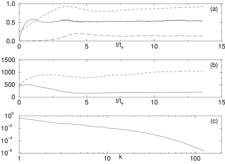
(a) skewness ( ), total energy ( ) and dissipation rate ( ); (b) microscale Reynolds number ( ) and integral scale Reynolds number ( ); (c) evolved energy spectrum. ( is the eddy turnover time)
We started from an existing, well validated code for the direct numerical simulation (DNS) of turbulence, constructed at the University of Edinburgh and running on the Cray T3D administered by the Edinburgh Parallel Computing Centre. In Figure 1 we have plotted a number of the standard DNS outputs generated by our code, running on a grid.
For the fundamentals of direct numerical simulations, the reader is directed to the pioneering work of Orszag (1969 and 1971). Time integration is performed by way of a second-order Runge-Kutta scheme and partial dealiasing is achieved through application of a random-shifting method (see, for example, Rogallo, 1981). At each time-step, the nonlinear term, , is calculated by a pseudospectral method involving a number of fast Fourier transforms. and may be computed by carrying out the same procedure having first zeroed the and fields respectively while may be calculated simply by subtracting and from the total nonlinear term.
Forcing
Stationarity is obtained by use of a deterministic forcing term given by,
| (17) |
where is the desired mean dissipation rate (supplied as an input parameter to the simulation), and
| (18) |
with defined as the energy spectrum. is chosen to be so that the forcing is applied to only the first shell of wavenumbers. With this forcing, we have observed over many simulations that after a sufficient number of time steps the velocity field reaches a statistically stationary form, as desired.
Computing the -fields
The evolution of and its partitions, as defined in equations (13)–(16), is a costly exercise as it must be performed in parallel with the evolution of the velocity field. We use a simple trapezoidal method to carry out the necessary time integrals, but the need to calculate each of the partitions of at each time step leads to a code that is roughly three times as computationally expensive as a straightforward DNS.
Further problems arise out of the necessity to choose suitable initial -fields with which to begin the computation. Here, we have chosen to begin by zeroing each of the -fields for all values of , in the expectation that after a sufficient number of time steps the initial conditions will have been forgotten. To this end, we run the DNS code until the four -fields have reached a statistically stationary state, and assume that this indicates convergence to their true values.

Further evidence may be provided by keeping in mind the fact that our forcing is only being applied to a single shell in wavenumber space, so that we have
| (19) |

with ( ) and ( ); with ( ) and ( ); with ( ) and ( ). The dot-dashed line indicates .

with ( ) and ( ); with ( ) and ( ); with ( ) and ( ). The dot-dashed line indicates .

with ( ) and ( ); with ( ) and ( ); with ( ) and ( ). The dot-dashed line indicates .

with ( ) and ( ); with ( ) and ( ); with ( ) and ( ). The dot-dashed line indicates .
We note that from our evolved data but carry out an additional test by computing the correlation between the two fields. We define the general correlation between two fields, and , by
| (20) |
and plot in Figure 2 for six different time steps. We see that by the final time step, the level of correlation is excellent for and good for . The increasing quality of correlation with increasing is to be expected as a consequence of the fact that higher wavenumbers evolve at a greater rate than lower wavenumbers — something which is borne out by looking at the correlations computed at earlier time steps. The deviation in the first shell is to be expected as this is outside the valid range of equation (19).
Finally we note that in order to compute -fields for different cutoff wavenumbers, , we must reperform the entire DNS from initial conditions up to the fully evolved state.
Experimental Details
We have computed -fields for a number of different cutoff wavenumbers at resolutions of and grid points. The high cost of calculating the -fields means that for these we have been restricted to a resolution of grid points and only two cutoff wavenumbers.
Our simulation achieved a microscale Reynolds number of while our simulation reached .
RESULTS
Low Reynolds Number
The results given in this section correspond to our simulation. We begin by presenting results for the -fields with cutoff wavenumbers and . Throughout this work, the cutoff wavenumbers are chosen to be half-integers so that they lie between two distinct shells. For each data set, we compute the correlation between and each of its partitions using equation (20) and also a measure of their relative magnitudes, , given by
| (21) |
Results are plotted in Figures 3 and 4, with both functions plotted against . We first note that, once scaled in this way, the exact choice of seems to have little effect on the shape of the graphs.

for cutoff wavenumbers , , , , , , with . The dot-dashed line indicates .

for cutoff wavenumbers , , , , , , with . The dot-dashed line indicates .

for cutoff wavenumbers , , , , , , with . The dot-dashed line indicates .

for cutoff wavenumbers , , , , , , with . The dot-dashed line indicates .

for cutoff wavenumbers , , , , , , with . The dot-dashed line indicates .

for cutoff wavenumbers , , , , , , with . The dot-dashed line indicates .
We believe that the peaky behaviour observed for in Figure 3 is an effect caused by the presence of the forcing term.
The general picture which seems to emerge from both correlation and magnitude information, is that for , the partition is the dominant part of . For , it is which is dominant while is broadly insignificant for all values of .
It was at this point in our work that it became apparent that the computational cost involved in calculating the -fields was too high and so attention was turned to the -fields which are far easier to calculate. For these, a single velocity field realization is enough to calculate and its partitions for any cutoff wavenumber, . We begin by duplicating the calculations performed on the -fields for the same resolution grid, and for the same cutoff wavenumbers. Results are shown in Figures 5 and 6 where we see a very similar picture to that presented in Figures 3 and 4.
Taking advantage of the reduction in computational effort, we now compute for a number of different cutoff wavenumbers. The results are shown in Figure 7. We see first of all that there is an excellent collapse of data for all cutoffs considered and that there is good correlation between and below the cutoff. Above the cutoff, this correlation decays rapidly away to zero. We also note that, mathematically, for so that the occurrence of a non-zero correlation in this region points to the existence of small numerical and aliasing errors.
This picture is reversed when we consider as shown in Figure 8. The collapse of data is not so good, particularly in the low-wavenumber region, and we see that as increases, the correlation begins to tail away from unity.
A pattern is even more difficult to discern when we compute , shown in Figure 9. We see that overall, does not correlate well with , although the level of correlation increases with as we move beyond the cutoff.
Moderate Reynolds Number
We now extend our work by applying the ideas outlined in previous sections to -field data from our simulations. Figures 10–12 show correlations of with each of its partitions from this data. As can be easily seen, the picture has changed very little from our data, the biggest difference being that the results seem better behaved, which is expected due to there being more data points available for shell averaging in the region .
In the following sections, all results are generated using the -fields taken from our simulation.
Eddy-viscosities with Sharp Cutoffs
We begin by rewriting our Navier-Stokes equation (6) for the low-wavenumber modes as
| (22) |
where the subscript ‘’ indicates that we are only concerned with and where
| (23) |
In a large eddy simulation, wavenumbers will not be available and so we introduce some model for which we will denote . A standard form for is an eddy-viscosity model, whereby
| (24) |
for some viscosity increment, .
We now consider a hypothetical large eddy simulation, based around the idea of our wavenumber cutoffs introduced in previous sections.
We can now compute the correlation between the exact subgrid terms and the model, . Because of ’s relationship with — and assuming only that is positive for all values of — this is equal to . The results are plotted in Figure 13. We see immediately that the correlation is, in general, quite poor. We also see what appears to be a difference in behaviour between cutoffs where there appears to be some degree of universality and cutoffs . In general, however, we can state quite categorically that, for the case of a sharp cutoff in wavenumber space, no eddy-viscosity model (subject to the reasonable constraint ) can perfectly reproduce the missing nonlinear terms. But, as we shall see, our conclusion will be modified somewhat when we consider phase and amplitude information separately.


Returning to equation (22), we can generate an energy balance equation by multiplying through by and averaging. Multiplying this through by then gives,
| (25) |
where describes energy transfer to and from the low-wavenumber modes through exclusively low-wavenumber couplings while describes energy transfer to and from the low-wavenumber modes through coupling involving at least one high-wavenumber mode. is the energy input due to the forcing. For interest’s sake, the two energy transfer functions are plotted in Figure 14. We see that has a large negative value in the first shell (note that the -axis has been truncated for this graph) corresponding to transfer of energy away from the energy input (forcing). We also see that is piling up energy at the cutoff and that this is balanced by which carries it to the higher wavenumbers.
Introducing an eddy-viscosity model as defined in equation (24) will give us an energy balance equation for LES,
| (26) |
Comparing equations (25) and (26) we can easily derive a form for the eddy viscosity,
| (27) |
For a large eddy simulation, this would ordinarily have to be estimated by use of some model, as the whole point of LES is the absence of the high-wavenumber modes necessary for the calculation of . However, with DNS data we can calculate this, and the results are plotted in Figure 15.
The general form of these eddy-viscosities appears to be in good agreement with the form obtained theoretically by, for example, Kraichnan (1976) and we know from previous work (see, for example, Lesieur and Rogallo, 1989) and our own LES experiments that this particular model provides good results. We must now ask why this is, when it is in apparent contradiction with the results presented in Figure 13.
Separating out Phase and Amplitude Effects
In this section we look at what happens if we separate our data into those contributions due to phase and those contributions due to amplitude. For each point in our field given by the wavevector, , we choose some unit vector perpendicular to which we call . We may then generate a transverse component of the velocity field,
| (28) |
We note that provides us with a statistically complete picture of our system. This is because, through continuity, , the component parallel to will be zero and due to isotropy, the statistical properties of are independent of the exact choice of .
Since we are working in Fourier space, will be a complex scalar and so may be rewritten in the form
| (29) |
and similarly for our -fields. We may now consider correlations based solely on phase or amplitude information (note that as we are now working with scalar fields, equation (20) must be modified by the removal of the sum over components, ).
In Figures 16—18 we have plotted correlations corresponding to Figures 10–12 but concerning ourselves only with phase information. We see a picture which is largely similar to that seen when considering all parts of the -fields, but note that in places — most obviously for in the data — the correlations are less good.
Moving on to Figures 19—21, where we have considered only amplitude information, we see a different picture. Here, while the regions of excellent correlation remain more or less untouched, for the rest of the data we see that the level of correlation does not drop below about and indeed seems to remain approximately constant at some value between and .
We can shed some light on the reasons for this by considering the statistical nature of the -fields. In Figures 22 and 23 we plot probability distribution functions for the amplitude and phase components respectively for each of the -fields11 1 We note that, strictly, these are not PDFs as our data set in this instance is insufficiently large — we would expect the true PDF of the phase components to be flat, for example. What we have instead is a measure of the distribution of that data which we do have.. We see that the possible values of the amplitude components are localised and similar in shape (in fact, for the chosen value of , the PDF’s for and are almost indistinguishable) and hence amplitude correlations will be good. On the other hand, there is no preferred phase and hence phase correlations will be very poor.
We now carry these ideas across to the analysis of general eddy viscosity models outlined in a previous section. Recall the definition of as a model for — we can now compare the phase and amplitude components of these two fields separately.
In Figure 24 we present the correlation obtained from phase information only and see that the general picture is the same as when we considered the whole fields. In Figure 25, however, where we consider only amplitude information, we see that there is uniformly good correlation at a level of around .

for cutoff wavenumbers , , , , , , with . The dot-dashed line indicates .

for cutoff wavenumbers , , , , , , with . The dot-dashed line indicates .

for cutoff wavenumbers , , , , , , with . The dot-dashed line indicates .

for cutoff wavenumbers , , , , , , with . The dot-dashed line indicates .

for cutoff wavenumbers , , , , , , with . The dot-dashed line indicates .

for cutoff wavenumbers , , , , , , with . The dot-dashed line indicates .
This means that the poor correlation between the exact subgrid terms and an eddy-viscosity model is due almost entirely to mismatching phases. However, by choosing suitably, it is possible to provide a good match as far as amplitude is concerned.


for cutoff wavenumbers ( ), ( ), ( ) with .
CONCLUSION
We have seen that, for the range of cutoff wavenumbers considered here, there is some degree of universal behaviour when we consider the partitions of the nonlinear term. We see that for , the terms involving coupling between low-wavenumber modes dominate, and this is a useful property when considering the potential for large eddy simulations. We have also seen that while it is not possible to represent subgrid terms exactly using an eddy-viscosity model, it is possible to model the amplitude of these terms. This will lead to reasonable results when one considers, for example, the flow of energy but it is clear that on a more fundamental level the velocity field will become corrupted due to phase-errors.
Acknowledgements: The results presented in this paper have been obtained from simulations performed on the computers of the Edinburgh Parallel Computing Centre. The research of A. Young is supported by the Engineering and Physical Sciences Research Council.

for cutoff wavenumbers ( ), ( ), ( ) with .
REFERENCES
Kraichnan, R.H., “Eddy viscosity in two and three dimensions,” J. Atmos. Sci., Vol. 33, pp. 1521–1536.
Lesieur, M. and Rogallo, R., 1989, “Large-eddy simulation of passive scalar diffusion in isotropic turbulence,” Phys. Fluids A, Vol. 1, No. 4, pp. 718–722.
McComb, W.D., 1995, “Theory of turbulence”, Rep. Prog. Phys., Vol. 58, pp. 1117-1206.
McComb, W. D., Roberts, W. and Watt, A. G., 1992, “Conditional-averaging procedure for problems with mode-mode coupling”, Phys. Rev. A, Vol. 45, pp. 3507–3515.
McComb, W. D. and Watt, A.G., 1992, “Two-field theory of incompressible-fluid turbulence”, Phys. Rev. A, Vol. 46, pp. 4797–4812.
McComb, W.D., Yang, T.-J., Young, A.J. and Machiels, L., 1997, “Investigation of renormalization group methods for the numerical simulation of isotropic turbulence,” Proc. 11th Symposium on Turbulent Shear Flows, Grenoble, pp. 4-23–4-27.
Machiels, L., 1997, “Predictability of small-scale motion in isotropic fluid turbulence,” Phys. Rev. Lett., Vol. 79, No. 18, pp. 3411–3414.
Orszag, S., 1969, “Numerical Methods for the Simulation of Turbulence,” Phys. Fluids (suppl. 2), Vol. 12, pp. 250–257.
Orszag, S., 1971, “Numerical Simulation of Incompressible Flows Within Simple Boundaries. I. Galerkin (Spectral) Representations,” Stud. Appl. Maths., Vol. 50, No. 4, pp. 293–327.
Rogallo, R.S., 1981, “Numerical Experiments in Homogeneous Turbulence,” NASA TM-81315.