Technical Report No. 9805, Department of Statistics, University of Toronto
Annealed Importance Sampling
Radford M. Neal
Department of Statistics and Department of Computer Science
University of Toronto, Toronto, Ontario, Canada
http://www.cs.utoronto.ca/radford/
radford@stat.utoronto.ca
| First version: | 18 February 1998 |
|---|---|
| Revised: | 1 September 1998 |
Abstract. Simulated annealing — moving from a tractable distribution to a distribution of interest via a sequence of intermediate distributions — has traditionally been used as an inexact method of handling isolated modes in Markov chain samplers. Here, it is shown how one can use the Markov chain transitions for such an annealing sequence to define an importance sampler. The Markov chain aspect allows this method to perform acceptably even for high-dimensional problems, where finding good importance sampling distributions would otherwise be very difficult, while the use of importance weights ensures that the estimates found converge to the correct values as the number of annealing runs increases. This annealed importance sampling procedure resembles the second half of the previously-studied tempered transitions, and can be seen as a generalization of a recently-proposed variant of sequential importance sampling. It is also related to thermodynamic integration methods for estimating ratios of normalizing constants. Annealed importance sampling is most attractive when isolated modes are present, or when estimates of normalizing constants are required, but it may also be more generally useful, since its independent sampling allows one to bypass some of the problems of assessing convergence and autocorrelation in Markov chain samplers.
1 Introduction
In Bayesian statistics and statistical physics, expectations of various quantities with respect to complex distributions must often be computed. For simple distributions, we can estimate expectations by sample averages based on points drawn independently from the distribution of interest. This simple Monte Carlo approach cannot be used when the distribution is too complex to allow easy generation of independent points. We might instead generate independent points from some simpler approximating distribution, and then use an importance sampling estimate, in which the points are weighted to compensate for use of the wrong distribution. Alternatively, we could use a sample of dependent points obtained by simulating a Markov chain that converges to the correct distribution. I show in this paper how these two approaches can be combined, by using an importance sampling distribution defined by a series of Markov chains.
This method is inspired by the idea of “annealing” as a way of coping with isolated modes, which leads me to call it annealed importance sampling. The method is especially suitable when multimodality may be a problem, but may be attractive even when it is not, since it allows one to bypass some of the problems of convergence assessment. Annealed importance sampling also supplies an estimate for the normalizing constant of the distribution sampled from. In statistical physics, minus the log of the normalizing constant for a canonical distribution is known as the “free energy”, and its estimation is a long-standing problem. In independent work, Jarzynski (1997a,b) has described a method primarily aimed at free energy estimation that is essentially the same as the annealed importance sampling method described here. I will focus instead on statistical applications, and will discuss use of the method for estimating expectations of functions of state, as well as the normalizing constant.
Importance sampling works as follows (see, for example, Geweke 1989). Suppose that we are interested in a distribution for some quantity, , with probabilities or probability densities that are proportional to the function . Suppose also that computing for any is feasible, but that we are not able to directly sample from the distribution it defines. However, we are able to sample from some other distribution that approximates the one defined by , whose probabilities or probability densities are proportional to the function , which we are also able to evaluate.
We base our estimates on a sample of independent points, , generated from the distribution defined by . For each , we compute an importance weight as follows:
| (1) |
We can then estimate the expectation of with respect to the distribution defined by by
| (2) |
Provided whenever , it is easy to see that will converge as to , where and are the normalizing constants for and . One can also see that will converge to the expectation of with respect to the distribution defined by .
The accuracy of depends on the variability of the importance weights. When these weights vary widely, the estimate will effectively be based on only the few points with the largest weights. For importance sampling to work well, the distribution defined by must therefore be a fairly good approximation to that defined by , so that the ratio does not vary wildly. When is high-dimensional, and is complex, and perhaps multimodal, finding a good importance sampling distribution can be very difficult, limiting the applicability of the method.
An alternative is to obtain a sample of dependent points by simulating a Markov chain that converges to the distribution of interest, as in the Metropolis-Hastings algorithm (Metropolis, et al 1953; Hastings 1970). Such Markov chain methods have long been used in statistical physics, and are now widely applied to statistical problems, as illustrated by the papers in the book edited by Gilks, Richardson, and Spiegelhalter (1996).
Markov chains used to sample from complex distributions must usually proceed by making only small changes to the state variables. This causes problems when the distribution contains several widely-separated modes, which are nearly isolated from each other with respect to these transitions. Because such a chain will move between modes only rarely, it will take a long time to reach equilibrium, and will exhibit high autocorrelations for functions of the state variables out to long time lags.
The method of simulated annealing was introduced by Kirkpatrick, Gelatt, and Vecchi (1983) as a way of handling multiple modes in an optimization context. It employs a sequence of distributions, with probabilities or probability densities given by to , in which each differs only slightly from . The distribution is the one of interest. The distribution is designed so that the Markov chain used to sample from it allows movement between all regions of the state space. A traditional scheme is to set , for .
An annealing run is started at some initial state, from which we first simulate a Markov chain designed to converge to , for some number of iterations, which are not necessarily enough to actually approach equilibrium. We next simulate some number of iterations of a Markov chain designed to converge to , starting from the final state of the previous simulation. We continue in this fashion, using the final state of the simulation for as the initial state of the simulation for , until we finally simulate the chain designed to converge to .
We hope that the distribution of the final state produced by this process is close to . Note that if contains isolated modes, simply simulating the Markov chain designed to converge to starting from some arbitrary point could give very poor results, as it might become stuck in whatever mode is closest to the starting point, even if that mode has little of the total probability mass. The annealing process is a heuristic for avoiding this, by taking advantage of the freer movement possible under the other distributions, while gradually approaching the desired . Unfortunately, there is no reason to think that annealing will give the precisely correct result, in which each mode of is found with exactly the right probability. This is of little consequence in an optimization context, where the final distribution is degenerate (at the maximum), but it is a serious flaw for the many applications in statistics and statistical physics that require a sample from a non-degenerate distribution.
The annealed importance sampling method I present in this paper is essentially a way of assigning weights to the states found by multiple simulated annealing runs, so as to produce estimates that converge to the correct value as the number of runs increases. This is done by viewing the annealing process as defining an importance sampling distribution, as explained below in Section 2. After discussing the accuracy of importance sampling in general in Section 3, I analyse the efficiency of annealed importance sampling in Section 4, and find that good results can be obtained by using a sufficient number of interpolating distributions, provided that these vary smoothly. Demonstrations on simple distributions in Section 5 and on a statistical problem in Section 6 confirm this.
Annealed importance sampling is related to tempered transitions (Neal 1996), which are another way of modifying the annealing procedure so as to produce correct results. As discussed in Section 7, annealed importance sampling will sometimes be preferable to using tempered transitions. When tempered transitions are still used, the relationship to annealed importance sampling allows one to find estimates for ratios of normalizing constants that were previously unavailable. Section 8 shows how one can also view a form of sequential importance sampling due to MacEachern, Clyde, and Liu (1998) as an instance of annealed importance sampling. Finally, in Section 9, I discuss the general utility of annealed importance sampling, as a way of handling multimodal distributions, as a way of calculating normalizing constants, and as a way of combining the adaptivity of Markov chains with the advantages of independent sampling.
2 The annealed importance sampling procedure
Suppose that we wish to find the expectation of some function of with respect to a distribution with probabilities or probability densities given by . We have available a sequence of other distributions, given by up to , which we hope will assist us in sampling from , and which satisfy wherever . For each distribution, we must be able to compute some function that is proportional to . We must also have some method for sampling from , preferably one that produces independent points. Finally, for each from to , we must be able to simulate some Markov chain transition, , that leaves invariant.
The sequence of distributions used can be specially constructed to suit the problem, but the following scheme may be generally useful. We fix to give the distribution of interest, and fix to give the simple distribution we can sample from, and then let
| (3) |
where . Note that the traditional simulated annealing scheme with would usually be less suitable, since it usually leads to a for which independent sampling is not easy.
For applications in Bayesian statistics, would be the prior density, which is often easy to sample from, and would be the unnormalized posterior distribution (the product of and the likelihood). When only posterior expectations are of interest, neither the prior nor the likelihood need be normalized. When the normalizing constant for the posterior (the marginal likelihood) is of interest, the likelihood must be properly normalized, but the prior need not be, as discussed below.
The Markov chain transitions are represented by functions giving the probability or probability density of moving to when the current state is . It will not be necessary to actually compute , only to generate an from a given using . These transitions may be constructed in any of the usual ways (eg, Metropolis or Gibbs sampling updates), and may involve several scans or other iterations. For the annealed importance sampling scheme to be valid, each must leave the corresponding invariant, but it is not essential that each produce an ergodic Markov chain (though this would usually be desirable).
Annealed importance sampling produces a sample of points, , and corresponding weights, . An estimate for the expectation of some function, , can then be found as in equation (2). To generate each point, , and associated weight, , we first generate a sequence of points, , as follows:
We then let , and set
| (10) |
To avoid overflow problems, it may be best to do the computations in terms of .
To see that annealed importance sampling is valid, we can consider an extended state space, with points . We identify with the original state, so that any function of the original state can be considered a function of the extended state, by just looking at only this component. We define the distribution for by the following function proportional to the joint probability or probability density:
| (11) |
Here, is the reversal of the transition defined by . That is,
| (12) |
The invariance of with respect to ensures that these are valid transition probabilities, for which . This in turn guarantees that the marginal distribution for in (11) is the same as the original distribution of interest (since the joint probability there is the product of this marginal probability for and the conditional probabilities for each of the later components given the earlier components).
For use below, we apply equation (12) to rewrite the function as follows:
| (13) | |||||
| (14) |
We now look at the joint distribution for defined by the annealed importance sampling procedure (2). It is proportional to the following function:
| (15) |
We regard this as an importance sampler for the distribution (11) on the extended state space. The appropriate importance weights are found using equations (1), (14), and (15). Dropping the superscript on the right side to simplify notation, they are:
| (16) |
These weights are the same as those of equation (10), showing that the annealed importance sampling procedure is valid.
The above procedure produces a sample of single independent points for use in estimating expectations as in equation (2). In practice, better estimates will often be obtained if we use each such point as the initial state for a Markov chain that leaves invariant, which we simulate for some pre-determined number of iterations. We can then estimate the expectation of by the weighted average (using the ) of the simple average of over the states of this Markov chain. This is valid because the expectation of with respect to is the same as the expectation with respect to of the average value of along a Markov chain that leaves invariant and which is started in state (since if the start state has distribution , all later states will also be from ).
Annealed importance sampling also provides an estimate of the ratio of the normalizing constants for and . Such normalizing constants are important in statistical physics and for statistical problems such as Bayesian model comparison. The normalizing constant for , as defined by equation (11), is the same as that for , and the normalizing constant for in equation (15) is the same as that for . The average of the importance weights, , converges to the ratio of these normalizing constants, , where and .
In a Bayesian application where is proportional to the prior and is the product of and the likelihood, the ratio will be the marginal likelihood of the model — that is, the prior probability or probability density of the observed data. Note that the prior need not be normalized, since any constant factors there will cancel in this ratio, but the likelihood must include all constant factors for this estimate of the marginal likelihood to be correct.
The data collected during annealed importance sampling runs from down to can also be used to estimate expectations with respect to any of the intermediate distributions, for . One simply uses the states, , found after application of in (2), with weights found by omitting the factors in equation (10) that pertain to later states. Similarly, one can estimate the ratio of the normalizing constants for and by averaging these weights.
Finally, although we would usually prefer to start annealing runs with a distribution from which we can generate independent points, annealed importance sampling is still valid even if the points generated at the start of each run are not independent. In particular, these points could be generated using a Markov chain that samples from . The annealed importance sampling estimates will still converge to the correct values, provided the Markov chain used to sample from is ergodic.
3 Accuracy of importance sampling estimates
Before discussing annealed importance sampling further, it is necessary to consider the accuracy of importance sampling estimates in general. These results will also be needed for the demonstrations in Sections 5 and 6.
For reference, here again is the importance sampling estimate, , for , based on points drawn independently from the density proportional to :
| (17) |
where are the importance weights.
The accuracy of this importance sampling estimator is discussed by Geweke (1989). An estimator of the same form is also used with regenerative Markov chain methods (Mykland, Tierney, and Yu 1995; Ripley 1987), where the weights are the lengths of tours between regeneration points.
In determining the accuracy of this estimator, we can assume without loss of generality that the normalizing constant for is such that , since multiplying all the by a constant has no effect on . We can also assume that , since adding a constant to simply shifts by that amount, without changing its variance. For large , the numerator and denominator on the right side of equation (17) will converge to their expectations, which on these assumptions gives
| (18) |
where and are the differences of the averages from their expectations. When is large, we can discard all but the first term, . We can judge the accuracy of by its variance (assuming this is finite), which we can approximate as
| (19) |
We now return to an actual situation, in which may not be one, and may not be zero, by modifying equation (19) suitably:
| (20) |
Geweke (1989) estimates this from the same data used to compute , as follows:
| (21) |
This is equivalent to the estimate discussed by Ripley (1987, Section 6.4) in the context of regenerative simulation. When is small, Ripley recommends using a jacknife estimate instead.
When and are independent under , equation (20) simplifies to
| (22) | |||||
| (23) |
The last step above uses the following:
| (24) | |||||
| (25) |
Equation (23) shows that when and are independent, the cost of using points drawn from rather than is given by one plus the variance of the normalized importance weights. We can estimate this using the sample variance of . This gives us a rough indication of the factor by which the sample size is effectively reduced, without reference to any particular function whose expectation is to be estimated. Note that in many applications the expectations of several functions will be estimated from the same sample of .
The variance of the is also intuitively attractive as an indicator of how accurate our estimates will be, since when it is large, the few points with the largest importance weights will dominate the estimates. It would be imprudent to trust an estimate when the adjusted sample size, , is very small, even if equation (21) gives a small estimate for the variance of the estimator. One should note, however, that it is possible for the sample variance of the to be small even when the estimates are wildly inaccurate, since this sample variance could be a very bad estimate of the true variance of the normalized importance weights. This could happen, for example, if an important mode of is almost never seen when sampling from .
Earlier, it was suggested that might be estimated by the weighted average of the values of over the states of a Markov chain that is started at each of the . The accuracy of such an estimate should be estimated by treating these average values for as single data points. Treating the dependent states from along the chain as if they were independently drawn from could lead to overestimation of the effective sample size.
Finally, if the are not independently drawn from , but are instead generated by a Markov chain sampler, assessing the accuracy of the estimates will be more difficult, as it will depend both on the variance of the normalized importance weights and on the autocorrelations produced by the Markov chain used. This is one reason for preferring a from which we can generate points independently at the start of each annealed importance sampling run.
4 Efficiency of annealed importance sampling
The efficiency of annealed importance sampling depends on the normalized importance weights, , not having too large a variance. There are several sources of variability in the importance weights. First, different annealing runs may end up in different modes, which will be assigned different weights. The variation in weights due to this will be large if some important modes are found only rarely. There is no general guarantee that this will not happen, and if it does, one can only hope to find a more effective scheme for defining the annealing distributions, or use a radically different Markov chain that eliminates the isolated modes altogether.
High variability in the importance weights can also result from using transitions for each of these distributions that do not bring the distribution close to equilibrium. The extreme case of this is when all the do nothing, in which case annealed importance sampling reduces to simple importance sampling based on , which will be very inefficient if is not close to . Variability from this source can reduced by increasing the number of iterations of the basic Markov chain update used. For example, if each consists of Metropolis updates, the variance of the importance weights might be reduced by increasing , so that brings the state closer to its equilibrium distribution, (at least within a local mode).
Variability in the importance weights can also come from using a finite number of distributions to interpolate between and , We can analyse how this affects the variance of the when the sequence of distributions used comes from a smoothly-varying one-parameter family, as in equation (3). For this analysis, we will assume that each produces a state drawn from , independent of the previous state. This assumption is of course unrealistic, especially when there are isolated modes, but the purpose here is to understand effects unrelated to Markov chain convergence.
It is convenient to look at rather than itself. As discussed in Section 3, we can measure the inefficiency of estimation by one plus the variance of the normalized importance weights. Using the fact that when and is Gaussian with mean and variance , we see that if the are Gaussian with mean and variance , the sample size will be effectively reduced by the factor
| (26) |
From equation (10),
| (27) |
If the distributions used are as defined by equation (3),
| (28) |
If we further assume that the are equally spaced (between 0 and 1), we have
| (29) |
Under the assumption that produces a state drawn independently from , and provided that has finite variance (when is drawn from ), the Central Limit Theorem can be applied to conclude that will have an approximately Gaussian distribution for large (keeping and fixed as increases). The variance of will asymptotically have the form , for some constant , and one plus the variance of the normalized weights will have the form . If we assume that each transition, , takes a fixed amount of time (regardless of ), the time required to produce an estimate of a given degree of accuracy will be proportional to , which is minimized when , at which point the variance of the logs of the importance weights will be one and the variance of the normalized importance weights will be .
The same behaviour will occur when the are not equally spaced, as long as they are chosen by a scheme that leads to going down approximately in inverse proportion to . Over a range of values for which is close to Gaussian, and is approximately constant in regions of high density under , an argument similar to that used for tempered transitions (Neal 1996, Section 4.2) shows that the best scheme uses a uniform spacing for (ie, a geometric spacing of the themselves). The results above also hold more generally for annealing schemes that are based on families of distributions for which the density at a given varies smoothly with a parameter analogous to .
We can get some idea of how the efficiency of annealed importance sampling will be affected by the dimensionality of the problem by supposing that under each , the components of are independent and identically distributed. Assuming as above that each produces an independent state drawn from , the quantities will be composed of identically distributed independent terms. The variance of each such quantity will increase in proportion to , as will the variance of , which will asymptotically have the form . The optimal choice of will be , which makes the variance of the normalized importance weights , as above. Assuming that behaviour is similar for more interesting distributions, where the components are not independent, this analysis shows that increasing the dimensionality of the problem will slow down annealed importance sampling. However, this linear slowdown is much less severe than that for simple importance sampling, whose efficiency goes down exponentially with .
The above analysis assumes that each generates a state nearly independent of the previous state, which would presumably require many Metropolis or Gibbs sampling iterations. It is probably better in practice, however, to use transitions that do not come close to producing an independent state, and hence take much less time, while increasing the number of interpolating distributions to produce the same total computation time. The states generated would still come from close to their equilibrium distributions, since these distributions will change less from one annealing step to the next, and the increased number of distributions may help to reduce the variance of the importance weights, though perhaps not as much as in the above analysis, since the terms in equation (29) will no longer be independent.
We therefore see that the variance of the importance weights can be reduced as needed by increasing the number of distributions used in the annealing scheme, provided that the transitions for each distribution are good enough at establishing equilibrium. When there are isolated modes, the latter provision will not be true in a global sense, but transitions that sample well within a local mode can be used. Whether the performance of annealed importance sampling is adequate will then depend on whether the annealing heuristic is in fact capable of finding all the modes of the distribution. In the absence of any theoretical information pointing to where the modes are located, reliance on some such heuristic is inevitable.
5 Demonstrations on simple distributions
To illustrate the behaviour of annealed importance sampling, I will show how it works on a simple distribution with a single mode, using Markov chain transitions that sample well for all intermediate distributions, and on a distribution with two modes, which are isolated with respect to the Markov chain transitions for the distribution of interest. Both distributions are over .
In the unimodal distribution, the six components of the state, to , are independent under , with the distribution for each being Gaussian with mean 1 and standard deviation 0.1. This distribution was defined by , whose normalizing constant is . A sequence of annealing distributions was defined according to the scheme of equation (3). Under the distribution chosen for , the components were independent, each being Gaussian with mean zero and standard deviation 1. The function used to define this distribution was chosen to be the corresponding Gaussian probability density, which was normalized. We can therefore estimate the normalizing constant for by the average of the importance weights.
To use annealed importance sampling, we must choose a sequence of that define the intermediate distributions. Both the number and the spacing of the must be appropriate for the problem. As mentioned in the previous section, for a Gaussian , and a diffuse , we expect that a geometric spacing will be appropriate for the that are not too far from one. I spaced the near zero arithmetically. In detail, for the first test, I used 40 spaced uniformly from 0 to 0.01, followed by 160 spaced geometrically from 0.01 to 1, for a total of 200 distributions. In later tests, annealing sequences with twice as many and half as many distributions were also used, spaced according to the same scheme.
We must also define Markov chain transitions, , for each of these distributions. In general, one might use different schemes for different distributions, but in these tests, I used Metropolis updates with the same proposal distributions for all (the transition probabilities themselves were of course different for each , since the Metropolis acceptance criterion changes). In detail, I used sequences of three Metropolis updates, with Gaussian proposal distributions centred on the current state having covariances of , , and . Used together, these three proposal distributions lead to adequate mixing for all of the intermediate distributions. For the first test, this sequence of three updates was repeated 10 times to give each ; in one later test, it was repeated only 5 times.
For each test, 1000 annealing runs were done. In the first test, 200 states were produced in each run, as a result of applying each in succession, starting from a point generated independently from . I saved only every twentieth state, however, after applying , , etc. down to . Note that was applied at the end of each run in these tests, even though this is not required (this occurs naturally with the program used). Only the state after applying was used for the estimates, even though it is valid to use the state after as well.
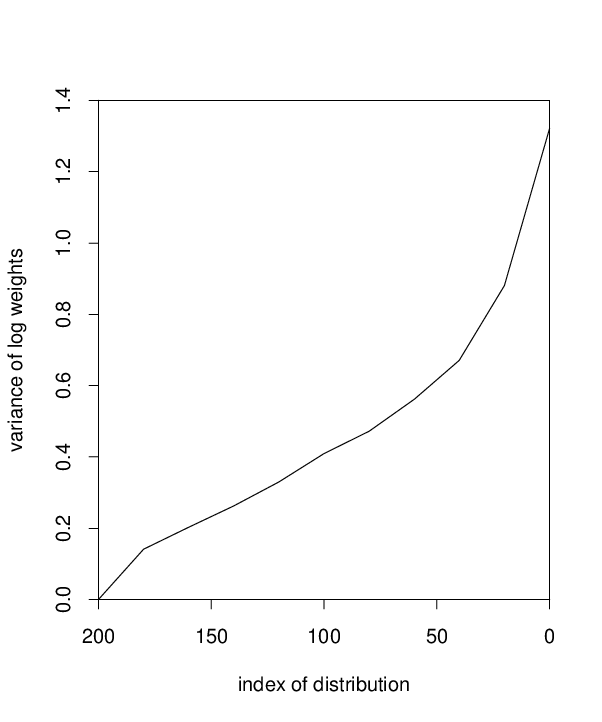
Figure 1 shows the results of this first test. The upper graphs show how the variance of the log of the importance weights increases during the course of a run. (Importance weights before the run is over are defined as in equation (10), but with the factors for the later distributions omitted.) When, as here, the transitions for all distributions are expected to mix well, the best strategy for minimizing the variance of the final weights is to space the so that the variance of the log weights increases by an equal amount in each annealing step. The plot in the upper right shows that the spacing chosen for this test is close to optimal in this respect. Furthermore, according to the analysis of Section 4, the number of intermediate distributions used here is close to optimal, since the variance of the logs of the weights at the end of the annealing run is close to one.
The lower two graphs in Figure 1 show the distribution of the value of the first component of the state () in this test. As seen in the lower left, this distribution narrows to the distribution under as approaches one. The plot in the lower right shows the values of the first component and of the importance weights for the states at the ends of the runs. In this case, the values and the weights appear to be independent.
The estimate for the expectation of the first component of the state in this first test is 1.0064, with standard error 0.0050, as estimated using equation (21). This is compatible with the true value of one. In this case, the error estimate from equation (21) is close what one would arrive at from the estimated standard deviation of 0.10038 and the adjusted sample size of , as expected when the values and the weights are independent. The average of the importance weights for this test was 0.000236, with standard error 0.000008 (estimated simply from the sample variance of the weights divided by ); this is compatible with the true normalizing constant of 0.000248.
Two tests were done in which each run used half as much computer time as in the first test. In one of these, the annealing sequence was identical to the first test, but the number of repetitions of the three Metropolis updates in each was reduced from 10 to 5. This increased the variance of the normalized importance weights to 2.18, with a corresponding increase in the standard errors of the estimates. In the other test, the number of distributions in the annealing sequence was cut in half (spaced according to the same scheme as before), while the number of Metropolis repetitions was kept at 10. This increased the variance of the normalized importance weights to 2.72. As expected, spreading a given number of updates over many intermediate distributions appears to be better than using many updates to try to produce nearly independent points at each of fewer stages.
The final test on this unimodal distribution used twice as many intermediate distributions, spaced according to the same scheme as before. This reduced the variance of the normalized importance weights to 0.461, with a corresponding reduction in standard errors, but the benefit in this case was not worth the factor of two increase in computer time. However, this test does confirm that when each mixes well, the variance of the importance weights can be reduced as desired by spacing the more closely.
Tests were also done on a distribution with two modes, which was a mixture of two Gaussians, under each of which the six components were independent, with the same means and standard deviations. One of these Gaussians, with mixing proportion , had means of 1 and standard deviations of 0.1, the same as the distribution used in the unimodal tests. The other Gaussian, with mixing proportion , had means of and standard deviations of 0.05. This mixture distribution was defined by the following :
| (30) |
The normalizing constant for this is . The means of the components with respect to this are .
The same as before was used for these tests (independent standard Gaussian distributions for each component, normalized). The same transitions based on Metropolis updates were used as well, along with the same scheme for spacing the . For the first test, the number of distributions used was 200, as in the first test on the unimodal distribution.
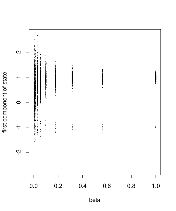
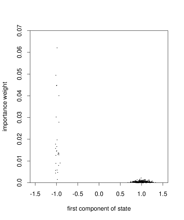
The results are shown in Figure 2. As seen in the lower left of the figure, the distributions for near zero cover both modes, but as is increased, the two modes become separated. The Metropolis updates are not able to move between these modes when is near one, even when using the larger proposals with standard deviation 0.5, since the probability of proposing a movement to the other mode simultaneously for all six components is very small. Both modes are seen when annealing, but the mode at is seen only rarely — 27 times in the 1000 runs — despite the fact that it has twice the probability of the other mode under the final distribution at . An unweighted average over the final states of the annealing runs would therefore give very inaccurate results.
The plot in the lower right of the figure shows how the importance weights compensate for this unrepresentative sampling. The runs that ended in the rarely-sampled mode received much higher weights than those ending in the well-sampled mode. The estimate for the expectation of the first component from these runs was , with an estimated standard error of 0.107 (from equation (21)), which is compatible with the true value of . This standard error estimate is less than one might expect from the estimated standard deviation of 0.92 and the adjusted sample size of , which was 35.0. The difference arises because the values and the importance weights are not independent in this case.


The average of the importance weights in these runs was 0.000766, with an estimated standard error of 0.000127, which is compatible with the true value of 0.000744 for the normalizing constant of .
We therefore see that annealed importance sampling produces valid estimates for this example. However, the procedure is less efficient than we might hope, because so few runs end in the mode at . Another symptom of the problem is that the variance of the normalized importance weights in this test was 27.6 — quite high compared to the variance of 1.12 seen in the similar test on the unimodal distribution. We can see how this comes about from the upper plots in Figure 2. For small values of , these plots are quite similar to those in Figure 1, presumably because the mode at has almost no influence for these distributions. However, this mode becomes important as approaches one, producing a high variance for the weights at the end.
One might hope to reduce the variance of the importance weights by increasing the number of intermediate distributions (ie, by spacing the more closely). I ran tests with twice as many distributions, and with four times as many distributions, in both cases using the same number of Metropolis updates for each distribution as before. The results differed little from those in the first test. The variance of the importance weights for runs ending within each mode was reduced, but the difference in importance weights between modes was not reduced, and the number of runs ending in the mode at did not increase. There was therefore little difference in the standard errors for the estimates.
For this example, the annealing heuristic used was only marginally adequate. One could expect to obtain better results only by finding a better initial distribution, , or a better scheme for interpolating from to than that of equation (3). This example also illustrates the dangers of uncritical reliance on empirical estimates of accuracy. If only 100 runs had been done, the probability that none of the runs would have found the mode at would have been around . This result can be simulated using the first 100 runs that ended in the mode at from the 1000 runs of the actual test. Based on these 100 runs, the estimate for the expectation of the first component is 0.992, with an estimated standard error 0.017, and the estimate for the normalizing constant of is 0.000228, with an estimated standard error of 0.000020. Both estimates differ from the true values by many times the estimated standard error. Such unrecognized inaccuracies are of course also possible with any other importance sampling or Markov chain method, whenever theoretically-derived guarantees of accuracy are not available.
6 Demonstration on a linear regression problem
To illustrate the use of annealed importance sampling for statistical problems, I will briefly describe its application to two Bayesian models for a linear regression problem, based on Gaussian and Cauchy priors. This example, and that of the previous section, are implemented using my software for flexible Bayesian modeling (version of 1998-09-01). The data and command files used are included with that software, which is available from my web page.
The data consists of 100 independent cases, each having 10 real-valued predictor variables, and a real-valued response variable, , which is modeled by
The residual, , is modeled as Gaussian with mean zero and unknown variance . The 100 cases were synthetically generated from this model with and with , , , and for . The predictor variables were generated from a multivariate Gaussian with the variance of each being one and with correlations of 0.9 between each pair of .
Two Bayesian models were tried. In both, the prior for the reciprocal of the residual variance () was gamma with mean and shape parameter . Both models also had a hyperparameter, , controlling the width of the distribution of the . Its reciprocal was given a gamma prior with mean and shape parameter . For the model with Gaussian priors, was the variance of the , which had mean zero, and were independent conditional on . The model based on Cauchy priors was similar, except that was the width parameter of the Cauchy distribution (ie, the density for conditional on was ). One might suspect that the Cauchy prior will prove more appropriate for the actual data, since this prior gives substantial probability to situations where many of the are close to zero, but a few are much bigger.
It seems quite possible that the posterior using the Cauchy prior could be multimodal. Since the are highly correlated, one can to some extent substitute for another. The Cauchy prior favours situations where only a few are large. This could produce several posterior modes that correspond to different sets of being regarded as significant.
I sampled for both models using a combination of Gibbs sampling for and the “hybrid Monte Carlo” method for the (see Neal 1996). There was no sign of any problems with isolated modes, but it is difficult to be sure on this basis that no such modes exist. Annealed importance sampling was applied in order to either find any isolated modes or provide further evidence of their absence, and also to compare the two models by calculating their marginal likelihoods.
An annealing schedule based on equation (3) was used. After some experimentation, adequate results were obtained using such a schedule with 1000 distributions: 50 distributions geometrically spaced from to , then 450 distributions geometrically spaced from to , and finally 500 distributions geometrically spaced from to . Hybrid Monte Carlo updates were used for each distribution. A single annealing run took approximately 8 seconds on our 194 MHz SGI machine. I did 500 such runs for each model.
Because a few of the annealing runs resulted in much smaller weights than others, the variance of the logs of the weights was very large, and hence was not useful in judging whether the annealing schedule was good. Instead, I looked at , the log of one plus the variance of the normalized importance weights. If the distribution of the logs of the weights were Gaussian, would be equal to the variance of the logs of the weights. When this distribution is not Gaussian, is less affected by a few extremely small weights. Plots of show that for both models it increases approximately linearly with the index of the distribution, reaching a final value around 0.6, only a bit less than the optimal value of one.
For both models, the estimates of the posterior means of the found using annealed importance did not differ significantly from those found using hybrid Monte Carlo without annealing. It therefore appears that isolated modes were not present in this problem. The annealed importance sampling runs yielded estimates for the log of the marginal likelihood for the model with Gaussian priors of -158.68 and for the model with Cauchy priors of -158.24, with a standard error of 0.04 for both estimates. The difference of 0.44 corresponds to a Bayes factor of 1.55 in favour of the model with Cauchy priors.
7 Relationship to tempered transitions
Several ways of modifying the simulated annealing procedure in order to produce asymptotically correct estimates have been developed in the past, including simulated tempering (Marinari and Parisi 1992; Geyer and Thompson 1995) and Metropolis coupled Markov chains (Geyer 1991). The method of tempered transitions (Neal 1996) is closely related to the annealed importance sampling method of this paper.
The tempered transition method samples from a distribution of interest, , using a Markov chain whose transitions are defined in terms of an elaborate proposal procedure, involving a sequence of other distributions, to . The proposed state is found by simulating a sequence of base transitions, to , which leave invariant the distributions to , followed by a second sequence of base transitions, to , which leave to invariant, and which are the reversals of the corresponding with respect to the . The decision whether to accept or reject the final state is based on a product of ratios of probabilities under the various distributions; if the proposed state is rejected, the new state is the same as the old state.
In detail, such a tempered transition operates as follows, starting from state :
The state is then accepted as the next state of the Markov chain with probability
| (40) |
The second half of the tempered transition procedure (7) is identical to the annealed importance sampling procedure (2), provided that in fact generates a point from that is independent of . We can also recognize that the annealed importance sampling weight given by equation (10) is essentially the same as the second half of the product defining the tempered transition acceptance probability (40). Due to these similarities, the characteristics of annealed importance sampling will be quite similar to those of the corresponding tempered transitions. In particular, the comparison by Neal (1996) of tempered transitions with simulated tempering is relevant to annealed importance sampling as well.
The major difference between annealed importance sampling and tempered transitions is that each tempered transition requires twice as much computation as the corresponding annealing run, since a tempered transition involves an “upward” sequence of transitions, from to , as well as the “downward” sequence, from to , that is present in both methods. This is a reason to prefer annealed importance sampling when it is easy to generate independent points from the distribution . When this is not easy, tempered transitions might be preferred, though annealed importance sampling could still be used in conjunction with a Markov chain sampler that produces dependent points from . With tempered transitions, there is also the possibility of using more than one sequence of annealing distributions (with the sequence chosen randomly for each tempered transition, or in some fixed order). Potentially, this could lead to good sampling even when neither annealing sequence would be adequate by itself. There appears to be no way of employing multiple annealing sequences with annealed importance sampling without adding an equivalent of the “upward” sequence present in tempered transitions.
When tempered transitions are used, the idea behind annealed importance sampling can be applied in order to estimate ratios of normalizing constants, which were previously unavailable when using tempered transitions. To see how to do this, note that the first half of a tempered transition (up to the generation of from using ) is the same as an annealed importance sampling run, but with the sequence of distributions reversed ( and exchange roles, the first state of the run is the current state, , which comes from , and in general, of (2) corresponds to of (7)). The importance weights for this backwards annealed importance sampling are
| (41) |
The average of these weights for all tempered transitions (both accepted and rejected) will converge to , the ratio of normalizing constants for and .
A similar estimate can be found by imagining the reversal of the Markov chain defined by the tempered transitions. In this chain, the states are visited in the reverse order, the accepted transitions of the original chain become accepted transitions in the reversed chain (but with the reversed sequence of states), and the rejected transitions of the original chain remain unchanged. An importance sampling estimate for the ratio of normalizing constants for and can be obtained using this reversed chain, in the same manner as above. The importance weights for the accepted transitions are as follows, in terms of the original chain:
| (42) |
The importance weights for the rejected transitions are the same as in equation (41). These two estimates can be averaged, producing an estimate that uses the states at both the beginning and the end of the accepted transitions, plus the states at the beginning of the rejected transitions, with double weight.
An estimate for the ratio of the normalizing constant for to that for can be found in similar fashion for any of the intermediate distributions, by simply averaging the weights obtained by truncating the products in equations (41) and (42) at the appropriate point. These weights can also be used to estimate expectations of functions with respect to these intermediate distributions. Note that error assessment for all these importance sampling estimates will have to take into account both the variance of the importance weights and the autocorrelations produced by the Markov chain based on the tempered transitions.
A cautionary note regarding these estimates comes from considering the situation when only two distributions are used, which are the prior and the posterior for a Bayesian model. The estimate for the reciprocal of the marginal likelihood based on equation (41) will then be the average over points drawn from the posterior of the reciprocal of the likelihood. This estimator will often have infinite variance, and will be very bad for any problem where there is enough data that the posterior is not much affected by the prior (since the marginal likelihood is affected by the prior). Compare this to the annealed importance sampling estimate for the marginal likelihood using just these two distributions, which will be the average of the likelihood over points drawn from the prior. This is not very good when the posterior is much more concentrated than the prior, but it is not as bad as averaging the reciprocal of the likelihood. Even when many intermediate distributions are used, it seems possible the annealed importance sampling estimates may be better than the corresponding “backwards” estimates using tempered transitions (assuming that is more diffuse than ).
8 Relationship to sequential importance sampling
A variant of sequential importance sampling recently developed by MacEachern, Clyde, and Liu (1998) can be viewed as an instance of annealed importance sampling, in which the sequence of distributions is obtained by looking at successively more data points.
This method (which MacEachern, et al call Sequential Importance Sampler S4) applies to a model for the joint distribution of observable variables along with associated latent variables (which have a finite range). We are able to compute these joint probabilities, as well as the marginal probabilities for the together with the over any subset of the indexes. We wish to estimate expectations with respect to the conditional distribution of given known values for . We could apply Gibbs sampling to this problem, but it is possible that it will be slow to converge, due to isolated modes.
The method of MacEachern, et al can be viewed as annealed importance sampling with a sequence of distributions, to , in which is related to the distribution conditional on of the observed variables; is then the distribution of interest, conditional on all of . In detail, these distributions have probabilities proportional to the following :
| (43) | |||||
We can apply annealed importance sampling with this sequence of distributions, using transitions defined as follows. begins with some number of Gibbs sampling updates for to , based only on . We can ignore to here because we can generate values for them afterward from their conditional distribution (under ) given to , independently of their previous values. This is done by forward simulation based on their conditional probabilities. (Actually, there is no need to generate values for with , since these values have no effect on the subsequent computations anyway.) This is easily seen to be equivalent to the sampling done in procedure S4 of MacEachern, et al.
The importance weights of equation (10) are products of factors of the following form:
| (44) | |||||
| (45) | |||||
| (46) | |||||
The product of these factors produces the same weights as used by MacEachern, et al.
Sequential Importance Sampler S4 of MacEachern, et al is thus equivalent to annealed importance sampling with the annealing distributions defined by equation (43). Unlike the family of distributions given by equation (3), these distributions form a fixed, discrete family. Consequently, the variance of the importance weights cannot be decreased by increasing the number of distributions. This could sometimes make the method too inefficient for practical use. However, it is possible that the sequence of distributions defined by equation (43) could be extended to a continuous family by partially conditioning on the in some way (eg, by adjusting the variance in a Gaussian likelihood). Other forms of annealed importance sampling (eg, based on the family of equation (3)) could also be applied to this problem.
9 Discussion
Annealed importance sampling is potentially useful as a way of dealing with isolated modes, as a means of calculating ratios of normalizing constants, and as a general Monte Carlo method that combines independent sampling with the adaptivity of Markov chain methods.
Handling isolated modes was the original motivation for annealing, and has been the primary motivation for developing methods related to annealing that produce asymptotically correct results. Annealed importance sampling is another such method, whose characteristics are similar to those of tempered transitions. As I have discussed (Neal 1996), which of these methods is best may depend on whether the sequence of annealing distributions is “deceptive” in certain ways. It is therefore not possible to say that annealed importance sampling will always be better than other methods such as simulated tempering, but it is probably the most easily implemented of these methods.
Annealing methods are closely related to methods for estimating ratios of normalizing constants based on simulations from many distributions, many of which are discussed by Gelman and Meng (1998). It is therefore not surprising that the methods of simulated tempering (Marinari and Parisi 1992; Geyer and Thompson 1995) and Metropolis coupled Markov chains (Geyer 1991) easily yield estimates for ratios of normalizing constants as a byproduct. Tempered transitions were previously seen as being deficient in this respect (Neal 1996), but we now see that such estimates can in fact be obtained by using annealed importance sampling estimators in conjunction with tempered transitions. One can also estimate expectations with respect to all the intermediate distributions in this way (as is also possible with simulated tempering and Metropolis coupled Markov chains).
Ratios of normalizing constants can also be obtained when using annealed importance sampling itself, which from this perspective can be seen as a form of thermodynamic integration (see Gelman and Meng 1998). One might expect a thermodynamic integration estimate based on a finite number of points to suffer from systematic error, but the results of this paper show that the annealed importance sampling estimate for the ratio of normalizing constants is in fact unbiased, and will converge to the correct value as the number of annealing runs increases. (Note that in this procedure one averages the estimates from multiple runs for the ratio of normalizing constants, not for the log of this ratio, as might perhaps seem more natural.)
Unlike simulated tempering and the related method of umbrella sampling (Torrie and Valleau 1977), no preliminary estimates for ratios of normalizing constants are required when using annealed importance sampling. Metropolis coupled Markov chains share this advantage, but have the disadvantage that they require storage for states from all the intermediate distributions. Annealed importance sampling may therefore be the most convenient general method for estimating normalizing constants.
In addition to these particular uses, annealed importance sampling may sometimes be attractive because it combines independent sampling with the ability of a Markov chain sampler to adapt to the characteristics of the distribution. Evans (1991) has also devised an adaptive importance sampling method that makes use of a sequence of intermediate distributions, similar to that used for annealing. His method requires that a class of tractable importance sampling densities be defined that contains a density appropriate for each of the distributions in this sequence. Annealed importance sampling instead uses a sampling distribution that is implicitly defined by the operation of the Markov chain transitions, whose density is generally not tractable to compute, making its use for simple importance sampling infeasible. From this perspective, the idea behind annealed importance sampling is that one can nevertheless find appropriate importance weights for use with this sampling distribution by looking at ratios of densities along the sequence of intermediate distributions.
One annoyance with Markov chain Monte Carlo is the need to estimate autocorrelations in order to assess the accuracy of the estimates obtained. Provided the points from used to start the annealing runs are generated independently, there is no need to do this with annealed importance sampling. Instead, one must estimate the variance of the normalized importance weights. This may perhaps be easier, though nightmare scenarios in which drastically wrong results are obtained without there there being any indication of a problem are possible when using methods of either sort. For annealed importance sampling, this can occur when the distribution of the importance weights has a heavy upward tail that is not apparent from the data collected.
Another annoyance with Markov chain Monte Carlo is the need to decide how much of a run to discard as “burn-in” — ie, as not coming from close to the equilibrium distribution. If only one, long run is simulated, the exact amount discarded as burn-in may not be crucial, but if several shorter runs are done instead, as is desirable in order to diagnose possible non-convergence, the decision may be harder. Discarding too little will lead to biased estimates; discarding too much will waste data. With annealed importance sampling, one must make an analogous decision of how much computation time to spend on the annealing runs themselves, which determine the importance weights, and how much to spend on simulating a chain that samples from starting from the final state from the annealing run (as is usually desirable, see Section 2). However, this decision affects only the variance of the estimates — the results are asymptotically correct regardless of how far the annealing process is from reaching equilibrium.
Regenerative methods (Mykland, Tierney, and Yu 1995) also eliminate the problems of dealing with sequential dependence (and also replace them with possible problems due to heavy-tailed distributions). To use regenerative methods, an appropriate “splitting” scheme must be devised for the Markov chain sampler. For high-dimensional problems, this may be harder than defining an appropriate sequence of intermediate distributions for use with annealed importance sampling.
As discussed in Section 4, the time required for annealed importance sampling can be expected to increase in direct proportion to the dimensionality of the problem (in addition to any increase due to the Markov chain samplers used being slower in higher dimensions). One must also consider the human and computer time required to select an appropriate sequence of intermediate distributions, along with appropriate Markov chain transitions for each. For these reasons, annealed importance sampling will probably be most useful when it allows one to find needed ratios of normalizing constants, or serves to avoid problems with isolated modes. One should note, however, that the potential for problems with multiple modes exists whenever there is no theoretical guarantee that the distribution is unimodal.
Acknowledgements
I thank David MacKay for helpful comments. This research was supported by the Natural Sciences and Engineering Research Council of Canada.
References
-
Evans, M. (1991) “Chaining via annealing”, Annals of Statistics, vol. 19, pp. 382-393.
-
Gelman, A. and Meng, X.-L. (1998) “Simulating normalizing constants: From importance sampling to bridge sampling to path sampling”, Statistical Science, vol. 13, pp. 163-185.
-
Geyer, C. J. (1991) “Markov chain Monte Carlo maximum likelihood”, in E. M. Keramidas (editor), Computing Science and Statistics: Proceedings of the 23rd Symposium on the Interface, pp. 156-163, Interface Foundation.
-
Geyer, C. J. and Thompson, E. A. (1995) “Annealing Markov chain Monte Carlo with applications to ancestral inference”, Journal of the American Statistical Association, vol. 90, pp. 909-920.
-
Geweke, J. (1989) “Bayesian inference in econometric models using Monte Carlo integration”, Econometrica, vol. 57, pp. 1317-1339.
-
Gilks, W. R., Richardson, S., and Spiegelhalter, D. J. (1996) Markov Chain Monte Carlo in Practice, London: Chapman and Hall.
-
Hastings, W. K. (1970) “Monte Carlo sampling methods using Markov chains and their applications”, Biometrika, vol. 57, pp. 97-109.
-
Jarzynski, C. (1997a) “Nonequilibrium equality for free energy differences”, Physical Review Letters, vol. 78, pp. 2690-2693.
-
Jarzynski, C. (1997b) “Equilibrium free-energy differences from nonequilibrium measurements: A master-equation approach”, Physical Review E, vol. 56, pp. 5018-5035.
-
Kirkpatrick, S., Gelatt, C. D., and Vecchi, M. P. (1983) “Optimization by simulated annealing”, Science, vol. 220, pp. 671-680.
-
Marinari, E. and Parisi, G. (1992) “Simulated tempering: A new Monte Carlo scheme”, Europhysics Letters, vol. 19, pp. 451-458.
-
MacEachern, S. N., Clyde, M., and Liu, J. S. (1998) “Sequential importance sampling for nonparametric Bayes models: The next generation”, to appear in The Canadian Journal of Statistics.
-
Metropolis, N., Rosenbluth, A. W., Rosenbluth, M. N., Teller, A. H., and Teller, E. (1953) “Equation of state calculations by fast computing machines”, Journal of Chemical Physics, vol. 21, pp. 1087-1092.
-
Mykland, C., Tierney, L., and Yu, B. (1995). “Regeneration in Markov Chain Samplers”, Journal of the American Statistical Association, vol. 90, pp. 233-241.
-
Neal, R. M. (1996) “Sampling from multimodal distributions using tempered transitions”, Statistics and Computing, vol. 6, pp. 353-366.
-
Neal, R. M. (1996) Bayesian Learning for Neural Networks, Lecture Notes in Statistics No. 118, New York: Springer-Verlag.
-
Ripley, B. D. (1987) Stochastic Simulation, New York: John Wiley.
-
Torrie, G. M. and Valleau, J. P. (1977) “Nonphysical sampling distributions in Monte Carlo free-energy estimation: Umbrella sampling“, Journal of Computational Physics, vol. 23, pp. 187-199.