Optimizing the Source Distribution in Fluid Mixing

Our goal is to maximize the enhancement factor $\mathcal{E}_{p}$ defined by (1),

where ${\widetilde{\theta}}$ solves equation (2) in the absence of advection,

with periodic boundary conditions on $[0,L]^{d}$. We assume that the velocity field is given. In maximizing the enhancement factor $\mathcal{E}_{p}$, we fix the $\mathrm{L}^{2}$ norm of the source and of the velocity field (or equivalently, the kinetic energy of the flow).

Define the linear operators

from which we can write the solution to (2) and (3) as

We can then rewrite the enhancement factor (1) as

where the self-adjoint operators $\mathcal{A}_{p}$ and ${\widetilde{}\mathcal{A}}_{p}$ are

and we have used the notation $\langle\cdot\rangle$ to denote integration over $[0,L]^{d}$. To maximize $\mathcal{E}_{p}^{2}$, we compute its variation with respect to $s$ and set it equal to zero,

which implies

or

This is an eigenvalue problem for the operator $\mathcal{K}_{p}\mathrel{\raisebox{0.29707pt}{:}\!\!=}\mathcal{A}_{p}{{\widetilde{}\mathcal{A}}_{p}}^{-1}$. The optimal source is given by the ground state of the inverse of this operator, and the normalized variance is given by the corresponding (first) eigenvalue.

The operators $\mathcal{A}_{p}^{-1}$ and ${\widetilde{}\mathcal{A}}_{p}^{-1}$ are self-adjoint from $\mathrm{L}^{2}([0,L]^{d})$ to $\mathrm{L}^{2}([0,L]^{d})$; furthermore, they are both positive operators in $\mathrm{L}^{2}([0,L]^{d})$ (restricted to functions with mean zero). Consequently, the generalized eigenvalue problem (7) has real positive eigenvalues, and the eigenfunctions $s$ and $s^{\prime}$ corresponding to distinct eigenvalues are orthogonal with respect to the weighted inner product $(s\,,\,s^{\prime})\mathrel{\raisebox{0.29707pt}{:}\!\!=}\langle s\,{\widetilde{}\mathcal{A}}_{p}^{-1}s^{\prime}\rangle$.

Our goal now is to calculate the optimal source and the corresponding mixing enhancement factor for some simple velocity fields. In particular, in Section III we will consider a weakly perturbed uniform flow in two dimensions, and in Section IV we will consider cellular flows. We will be primarily concerned with the eigenvalue problem (7) or (8) for $p=0$, i.e.

with $\mathcal{A}\mathrel{\raisebox{0.29707pt}{:}\!\!=}\mathcal{A}_{0}={\mathcal{L}}{\mathcal{L}}^{*},\,{\widetilde{}\mathcal{A}}\mathrel{\raisebox{0.29707pt}{:}\!\!=}{\widetilde{}\mathcal{A}}_{0}=\kappa^{2}\Delta^{2}$ and $\mathcal{E}\mathrel{\raisebox{0.29707pt}{:}\!\!=}\mathcal{E}_{0}$. Notice that the operator ${\widetilde{}\mathcal{A}}^{-1}$ is a diagonal operator in Fourier space with entries $\kappa^{2}\lvert{\bm{k}}\rvert^{-4}$, where ${\bm{k}}$ is the wavevector. The large negative power of $\lvert{\bm{k}}\rvert$ indicates that this operator acts as a low-pass filter, suppressing high frequencies. We shall return to the case $p\neq 0$ in Section IV.3.

Before considering specific examples in Sections III and IV, let us demonstrate that the optimal solution obtained in Section II.1 is indeed a global maximum. We could do this using the second variation of $\mathcal{E}_{p}^{2}$, but instead we proceed more directly by expanding an arbitrary source in terms of eigenfunctions $s^{(i)}$ satisfying Eq. (7),

and inserting into expression (4) for the mixing enhancement factor,

where we used the eigenfunction property. Now use the orthogonality property of the $s^{(j)}$, $\langle s^{(i)}\,{\widetilde{}\mathcal{A}}_{p}^{-1}s^{(j)}\rangle=\delta_{ij}$, and the fact that ${\mathcal{E}_{p}}\geq{{\mathcal{E}_{p}^{(j)}}}$, that is the optimal enhancement factor $\mathcal{E}_{p}$ is the largest eigenvalue, to find

which proves that $\mathcal{E}_{p}$ is indeed optimal, since the enhancement factor of no other source can exceed it. This is a global argument, which relies only on the eigenvalue problem (7) providing a complete set of orthogonal eigenfunctions.

For completeness, in this short section we essentially rederive the results of Plasting and Young 2006, Doering and Thiffeault 2006, and Shaw et al. 2007 on the optimality of a uniform flow. We start with a time-independent spatially uniform flow on $[0,L]^{d}$,

From definition (5) with $p=0$, we have that

and

Since $\mathcal{K}$ is a differential operator with constant coefficients on a periodic domain, its eigenfunctions are easily verified to be

where ${\bm{k}}$ is the wavevector and $\hat{s}_{\bm{k}}$ is a normalization constant, and the corresponding eigenvalues are

We can maximize the above expression by choosing ${\bm{k}}$ to be the shortest allowable vector parallel to the uniform flow $\bm{U}$. (Not all magnitudes and directions are allowed for wavevectors because the domain is periodic: the components of ${\bm{k}}$ are integer multiples of $2\pi/L$.)

In the particular case where the uniform flow $\bm{U}$ is along the $x$–axis, $\bm{U}=U\,{\hat{\bm{e}}_{x}}$, we have that

where we have defined the Péclet number $\mathrm{Pe}\mathrel{\raisebox{0.29707pt}{:}\!\!=}UL/2\pi\kappa$. As expected, in the limit as $\kappa\rightarrow\infty$ ($\mathrm{Pe}\rightarrow 0$), the mixing enhancement factor converges to $1$, i.e. in the large diffusivity limit the enhancement due to a flow becomes negligible. On the other hand, in the limit $\kappa\rightarrow 0$ ($\mathrm{Pe}\rightarrow\infty$) the enhancement factor grows like $\kappa^{-1}$.

Consider now a two-dimensional uniform flow along the $x$–axis perturbed by a weak flow,

with $\varepsilon\ll 1$ and $\langle\bm{u}_{1}\rangle=0$. The second-order term is included to make ${\lVert\bm{u}\rVert}_{2}=U+\mathrm{O}(\varepsilon^{4})$, so that we can compare the effect of the perturbed and unperturbed flows at equal amplitude. Specifically, we consider perturbations of the form

which are simple to analyze but yield important insight. Because the base flow is in the ${\hat{\bm{e}}_{x}}$ direction, the $u_{1x}(y){\hat{\bm{e}}_{x}}$ term is a shear flow perturbation, and the $u_{1y}(x){\hat{\bm{e}}_{y}}$ term is a wavy flow perturbation. Our goal is to obtain an asymptotic expansion for the optimal source and enhancement factor. For this we need to study perturbatively the eigenvalue problem (9), which we write as

with $\mathcal{A}={\mathcal{L}}{\mathcal{L}}^{*}$, ${\widetilde{}\mathcal{A}}=\widetilde{}{\mathcal{L}}\widetilde{}{\mathcal{L}}^{*}=\kappa^{2}\Delta^{2}$, and $\lambda=\mathcal{E}^{2}$. We have that

with

where $u_{2x}$ is the coefficient of the second-order term in (13). Consequently,

Note that in this section the subscripts on the $\mathcal{A}$’s correspond to their order in $\varepsilon$, and not to the $p$ subscript as in Eq. (5) (recall that $p=0$ for the present section). We expand $s$ and $\lambda$ in a power series in $\varepsilon$,

insert the expansions for $\mathcal{A},\,s$ and $\lambda$ in equation (14), and equate like powers of $\varepsilon$ to obtain the sequence of equations

Consider first equation (15a), the unperturbed equation: from Section III.1 we have that

where $k_{0}\mathrel{\raisebox{0.29707pt}{:}\!\!=}2\pi/L$. We proceed now with equation (15b): multiply by $s_{0}$ and integrate over $[0,L]^{2}$ to obtain

Notice that $\mathcal{A}_{0}$ is a differential operator with constant coefficients, and hence it commutes with ${\widetilde{}\mathcal{A}}^{-1}$. Furthermore, both operators are self-adjoint, so that

and equation (16) simplifies to

leading to

where the last equality follows from a straightforward calculation. This is a consequence of the invariance of the enhancement factor under reversal of the pertubation, from which all odd powers of $\varepsilon$ in the enhancement factor will vanish.

Now we compute $s_{1}$. We set $\lambda_{1}=0$ in equation (15b) to obtain

For definiteness, we specify the form of the perturbation,

Notice that we do not yet need to specify $u_{1y}(x)$: it only affects the result at the next order. We look for a solution to (18) in the form of

and find

Let us proceed now with the calculation of $\lambda_{2}$. We multiply (15c) by $s_{0}$, integrate over $[0,L]^{2}$ and use (17) to obtain

which after substituting our solution (19)–(20) for $s_{1}$ simplifies to

We are really after the enhancement factor, which is

so after putting it all together, we can write $\mathcal{E}$ in terms of dimensionless quantities,

where $\alpha\mathrel{\raisebox{0.29707pt}{:}\!\!=}k_{1}/k_{0}$ and recall that $\mathrm{Pe}=U/\kappa k_{0}$.

Some observations regarding (21) are in order. First, notice that a nonzero $u_{1x}$ (shear flow perturbation) increases the enhancement factor, while a nonzero $u_{1y}$ (wavy flow) decreases it. Second, the form of $u_{1y}$ is irrelevant, and it does not affect the first-order optimal source distribution. Third, in the limit of large $\kappa$ (small $\mathrm{Pe}$), the $\mathrm{Pe}^{-2}$ term in (21), arising from $\kappa^{2}\Delta^{2}$ in $\mathcal{A}_{0}$, invalidates the expansion. We discuss each type of perturbation in turn.

Figure 1 shows the optimal source distribution for $U=1$, $L=2\pi$, $\kappa=0.01$ ($\mathrm{Pe}=100$), $\hat{u}_{1x}=1/\sqrt{2}$, $k_{1}=2$, $\varepsilon=0.15$, $u_{1y}=0$.

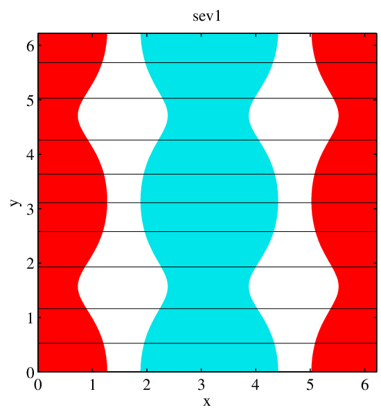
This is a shear flow, with contour lines shown in the background. The contour lines are closer together at the midpoint, indicating faster flow, since the perturbation is $u_{1x}(y)=\sqrt{2}\cos 2y$. Accordingly, the optimal source is localized at these points of faster flow. However, there is a limit to how localized it can get: if the source were to bunch up too much in the faster region, the purely-diffusive solution would be more effective (i.e., have lower variance), reducing the enhancement factor. As the perturbation gets larger, the optimal source will bunch up more in the faster regions, since the gain becomes greater. The enhancement factor is always greater than in the unperturbed case, suggesting that the advantage of faster flow regions outweighs the disadvantage of localizing the source. Finally, note that for large $\alpha$ (large perturbation wavenumber $k_{1}$), the mixing enhancement factor becomes independent of $\alpha$, reflecting the fact that a fine-scale perturbation is overwhelmed by diffusion.

Conversely, Figure 1 shows the optimal source distribution for the same parameters as the shear flow above but with perturbation $u_{1y}=\sqrt{2}\cos 2x$, $u_{1x}=0$. The streamlines in the background indicate that this is a wavy flow, with no dependence on $y$. The optimal source distribution, again shown in the background (here as $\cos x$, but the phase is arbitrary), is exactly the same as in the absence of perturbation. Intuitively, one could expect the source to be more efficient if it tilted to present its contours perpendicular to the flow, giving a wavy source. This is not the case, since the purely-diffusive solution would be more effective for a wavy source, and thus lower the enhancement factor since it enters the numerator in the definition (1). Localizing the source in regions of faster flow (as for the perturbation in Fig. 1) is a more important effect than aligning the contours of the source perpendicular to the flow.

We consider the perturbed cellular flow with streamfunction

with velocity field $\bm{u}=(u_{x},u_{y})=(\partial_{y}\psi,-\partial_{x}\psi)$, where $A$ is a normalization constant chosen to make $\lVert\bm{u}\rVert_{2}=1$. With $\delta_{1}=\delta_{2}=0$ (the basic cellular flow), the operator ${\mathcal{L}}$ is invariant under the discrete symmetry group $\mathcal{G}$ generated by the transformations

The Abelian group $\mathcal{G}$ has order $8$ and is characterized by $G_{1}^{4}=G_{2}^{2}=I$, $G_{1}G_{2}=G_{2}G_{1}$.¹¹ 1 $\mathcal{G}$ is the direct product of a cyclic group of order 4 and a cyclic group of order 2. For either $\delta_{1}$ or $\delta_{2}$ nonzero, the perturbations break the symmetry $G_{1}$ of the cellular flow, and we shall look at their effect in turn.

First we set $\delta_{1}=\delta_{2}=0$ in (23) and solve (22) with $\kappa=0.01$.

In this case, there are two independent optimal source eigenfunctions with degenerate enhancement factor $\mathcal{E}=87.34$, shown in Fig. 2. In the foreground are contour lines of the streamfunction. Any superposition of the two eigenfunctions in Fig. 2 will give the same enhancement factor. The degeneracy is a consequence of the symmetry $G_{1}$ of the cellular flow: indeed, the two eigenfunctions are related to each other (up to a sign) by the transformation (24a). The two eigenfunctions also separately have the $G_{2}$ symmetry. This situation, where the eigenfunctions corresponding to the same eigenvalue are related by a unitary representation of the symmetry group of an operator, is familiar from quantum mechanics Wigner 1959; Hamermesh 1989.

For comparison, the enhancement factor for the same flow but with the reference source $s(\bm{x})=\sin x$ is $50.01$, and with the reference source $\cos x$ is $86.61$. Hence, for $\sin x$ the optimal source gives a $74.7\%$ improvement in the enhancement factor, but only $0.9\%$ for $\cos x$. It is remarkable how close $\cos x$ comes to the optimal enhancement factor, which shows that the optimal source is rather ‘robust’, so that small changes in its shape do not lead to huge changes in the enhancement factor. From a design standpoint, this is highly desirable. Table 1 summarizes the optimal enhancement factor results for different values of the perturbations $\delta_{1}$ and $\delta_{2}$.

How to interpret the optimal source distribution in Fig. 2? The lesson learned from the uniform flow of Section III is that, ideally, the source should be such that the velocity field advects heat from hot to cold and vice versa. This is clearly happening in Fig. 2 to some extent, since in both eigenfunctions the hot and cold spots are situated such that the rolls easily advect heat between hot and cold. However, this is not the whole story: the optimal source is also distributed so as to take advantage of regions of faster flow. This is readily apparent in Fig. 3, which shows the magnitude of the velocity field in the background,

and contours of the optimal source distribution from Fig. 2 (right). The hot and cold spots (elliptic regions) are clearly localized over the regions of rapid flow (pale background). Some of the fast regions appear to have no hot or cold spots, but these regions are favored in the other eigenfunction, so the symmetry is respected.

Next, we resolve the degeneracy of the optimal source distribution by setting $\delta_{1}=0.05$ in (23) while keeping $\delta_{2}=0$, giving the streamfunction shown as contour lines in the foreground of Fig. 4. The rolls now have a slight asymmetry that breaks the rotational symmetry $G_{1}$ of the unperturbed cellular flow. As a consequence, the normalized optimal eigenfunction is now unique, and is shown as the shaded background in Fig. 4. It is very close to the degenerate eigenfunction on the right in Fig. 2, and converges to it as $\delta_{1}\rightarrow 0$. The enhancement factor in this case is almost unchanged, $87.59$. Again, the cosine reference source has much higher enhancement factor ($86.18$, $1.6\%$ improvement for the optimal source) than the sine reference source ($49.76$, $76.0\%$ improvement for the optimal source).

Finally, we set $\delta_{1}=0$ and $\delta_{2}=0.05$ in (23), with the streamfunction shown as contours in the foreground of Fig. 4. As for the previous perturbation, this one also breaks the $G_{1}$ symmetry and causes the optimal eigenfunction to become unique, but this time a superposition of the two degenerate eigenfunctions in Fig. 2 is selected. The optimal enhancement factor, $90.10$, is again almost unchanged by this small perturbation.

To summarize this section, we presented three cases at fixed diffusivity $\kappa=0.01$. The first was the cellular flow, for which we get doubly-degenerate optimal eigenfunctions. We then presented two symmetry-breaking perturbations in turn, showing how these select a particular mixture of the degenerate eigenfunctions to create a unique optimal source distribution. Since the perturbations are small, the optimal enhancement factor in all these cases is about the same, showing an improvement of about $75$–$80\%$ over the reference source $\sin x$, but only $1$–$5\%$ over the reference source $\cos x$. This latter modest improvement is best seen not as a failure of the optimization procedure, but as an advantage, since robustness is always desirable. In fact robustness can easily be gauged by looking at the magnitude of the next largest eigenvalues, to see how far they are from the dominant one(s). Table 1 also shows that the modest improvement over the cosine source is an accident, since for many other velocity fields improvements well above $50\%$ are seen for both sine and cosine. Two further examples for large perturbations are shown in Figs. 4 and 4.

Now we will fix $\delta_{1}=\delta_{2}=0$ in (23) and vary the diffusivity, $\kappa$. For $\kappa=0.01$, Fig. 2 shows the two degenerate optimal source eigenfunctions, and we will follow the change in the one on the left as $\kappa$ is varied. In Fig. 5 we show the

change in the optimal source as $\kappa$ is increased from $0.1$ to $100$. The optimal source distribution appears to become independent of $\kappa$ both for small $\kappa$ and large $\kappa$, but the distributions are different. The transition between the two regimes occurs when $\kappa$ is of order unity. Though the two asymptotic sources are very different, they respect the general principles laid out in Section IV.1: the source is arranged for effective transport of hot onto cold and vice versa, and regions of high speed are favored. In particular, note that the center of the rolls has a nearly zero, flat source distribution in all cases.

Another perhaps surprising aspect of the large $\kappa$ solution in Fig. 5 is that it has complicated structure. In this large diffusivity limit, one would expect diffusion to dominate and gradients to be smoothed out. But since our mixing enhancement factor (1) compares the variance to the unstirred case, which already has very low variance, any amount of improvement will count. Hence, the complicated source for large $\kappa$ in Fig. 5 only gives a minute improvement to the enhancement factor. The large $\kappa$ optimal solution is particular in that it has some hot and cold spots localized over hyperbolic stagnation points. This is probably due to the high speeds along the separatrices being favored, even at the cost of straddling hyperbolic stagnation points a little.

Figure 6 shows how the mixing enhancement factor varies as a function of the diffusivity.

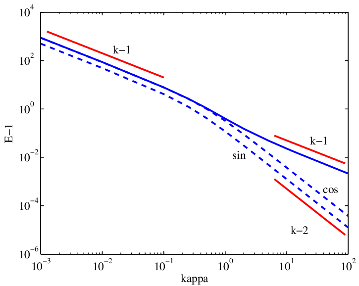
The solid line is for the optimal source, the dashed lines for the reference sources $\sin x$ and $\cos x$. For small $\kappa$, the enhancement factor of all sources scales as $\kappa^{-1}$: this is the ‘classical’ scaling discussed in Thiffeault et al. 2004; Doering and Thiffeault 2006; Shaw et al. 2007, where the enhancement factor is linear in the Péclet number. It has been rigorously proved in Thiffeault et al. 2004; Doering and Thiffeault 2006; Shaw et al. 2007 that this scaling is optimal over all possible sources and velocity fields.

For $\kappa$ near unity, the optimal enhancement factor has a small dip before converging towards unity as $\kappa^{-1}$ for large $\kappa$. In contrast, the reference enhancement factors converges to unity as $\kappa^{-2}$. This last scaling holds for the uniform flow of Section III when expanded in large $\kappa$, and is verified for other flows and sources as well Thiffeault et al. 2004; Doering and Thiffeault 2006; Shaw et al. 2007.

In summary, the optimal source distribution becomes independent of $\kappa$ for both large and small $\kappa$, but of course for large $\kappa$ the efficiency gain is minimal (since the $\mathrm{L}^{2}$–norm of the velocity is fixed). For small $\kappa$ the efficiency gain is a constant multiple of the reference sources, but this multiple is fairly small for $\cos x$ ($1.01$), showing that optimization is very robust but not necessarily always worthwhile. Overall, the optimal enhancement factor scales as $\kappa^{-1}$, with a momentary break in the scaling that corresponds to the complicated change in topology seen in Fig. 5 for $\kappa$ near unity.

Our final study will be to examine the behavior of the optimal enhancement factor as $p$ is varied in (1). In Sections IV.1–IV.2 we used $p=0$; now we fix $\delta_{1}=\delta_{2}=0$, $\kappa=0.01$, and allow $p$ to vary over negative and positive values.

Figure 7 shows the optimal source distributions for $p$ varying from $-1$ to $2$. For both negative and positive $p$, the optimal source distribution converges rapidly to invariant patterns, and the two extremes in Fig. 7 are representative of those asymptotic patterns. The situation is thus entirely analogous to the case where diffusivity was varied (Fig. 5).

The top-left picture in Fig. 7 (negative $p$) shows small, localized sources and sinks. In contrast, the bottom-right picture in Fig. 7 (positive $p$) shows large, regular localized sources and sinks. In fact, what is striking about the pattern is its simplicity: it is what one might take as a guess at an efficient source distribution, with no added frills. Thus, a high power of $p$ might be useful in situations where a simple configuration is necessary due to engineering constraints. The reason for the simplicity is that spatial variations in the source favor the diffusion operator in ${\mathcal{L}}$, and as $p\rightarrow\infty$ these are magnified. Thus, the source must remain as spatially simple as possible while trying to maximize alignment with the velocity. As $p\rightarrow-\infty$, spatial variations of the source are downplayed by the norm, allowing more complexity.

Figure 8 shows how the optimal mixing enhancement factor

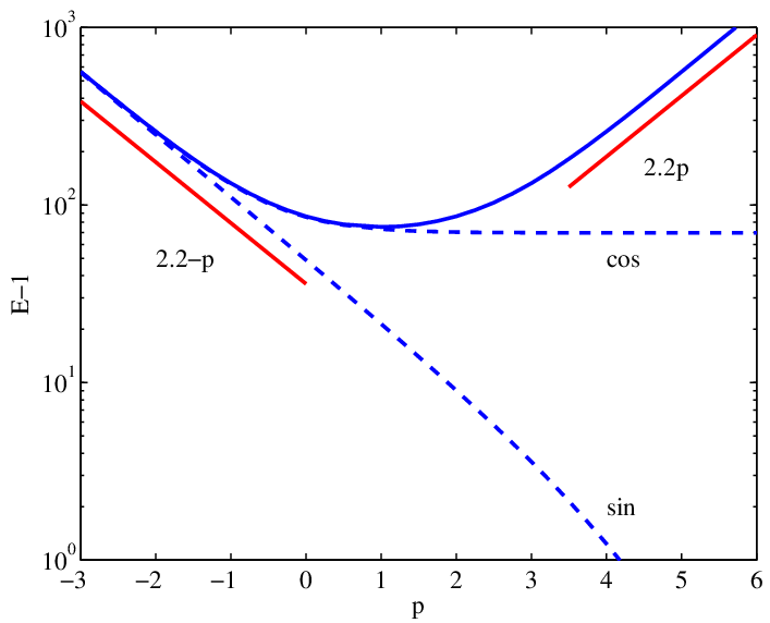
varies as a function of $p$. For $p\rightarrow-\infty$, the enhancement factor goes to infinity, as does the enhancement factor of the two reference sources. For $p\rightarrow\infty$, the enhancement factor also goes to infinity, but the reference source enhancement factors now approach constants (the constant is $1$ for $\sin x$). Again, we are seeing the effect of the diffusion term dominating when gradients are present, since these are amplified by $(-\Delta)^{p/2}$. Note that the curve is symmetric about $p=1$, which leads to a minimum there: whether this is true in general has not been determined, but we have not found a counterexample. In Appendix A we provide a partial proof by explicitly finding the symmetry between the operators $\mathcal{A}_{2-p}$ and $\mathcal{A}_{p}$, but only for large $\kappa$.