Undulator Radiation in a Waveguide
Abstract
We propose an analytical approach to characterize undulator radiation near resonance, when the presence of the vacuum-pipe considerably affects radiation properties. This is the case of the far-infrared undulator beamline at the Free-electron LASer (FEL) in Hamburg (FLASH), that will be capable of delivering pulses in the TeraHertz (THz) range. This undulator will allow pump-probe experiments where THz pulses are naturally synchronized to the VUV pulse from the FEL, as well as the development of novel electron-beam diagnostics techniques. Since the THz radiation diffraction-size exceeds the vacuum-chamber dimensions, characterization of infrared radiation must be performed accounting for the presence of a waveguide. We developed a theory of undulator radiation in a waveguide based on paraxial and resonance approximation. We solved the field equation with a tensor Green’s function technique, and extracted figure of merits describing in a simple way the influence of the vacuum-pipe on the radiation pulse as a function of the problem parameters. Our theory, that makes consistent use of dimensionless analysis, allows treatment and physical understanding of many asymptotes of the parameter space, together with their region of applicability.
Keywords:
Synchrotron Radiation , Near Field , Passive Waveguide , Tensor Green’s Function , Undulator RadiationPACS
41.60.Ap , 41.60.-m , 41.20.-qDEUTSCHES ELEKTRONEN-SYNCHROTRON
in der HELMHOLTZ-GEMEINSCHAFT
DESY 07-031
March 2007
Undulator Radiation in a Waveguide
Gianluca Geloni, Evgeni Saldin, Evgeni Schneidmiller and Mikhail Yurkov
Deutsches Elektronen-Synchrotron DESY, Hamburg ISSN 0418-9833 NOTKESTRASSE 85 - 22607 HAMBURG
1 Introduction
At the start of this century we have seen a revolution in synchrotron source intensities. This revolution stemmed from the technique of Free-Electron Lasers (FELs), combined with recent progress in accelerator technology, developed in connection with high-energy linear colliders.
A new era of Synchrotron Radiation research has begun with first user experiments on VUV-FEL, based on Self-Amplified Spontaneous Emission (SASE) NEW1, NEW2. These results have been obtained at the TESLA (Tera Electronvolt Superconducting Linear Accelerator) Test Facility (TTF) at Deutsches Elektronen-SYnchrotron (DESY) at Hamburg, Germany. Radiation pulses with a wavelength of nm, fs duration and GW peak power where used at TTF, phase NEW3, NEW4.
This facility is now called FLASH (Free-Electron LAser in Hamburg), and operates as a user facility since August 2005 NEW5, NEW6. Currently FLASH produces GW-level, laser-like VUV (Vacuum Ultra-Violet) to EUV (Extreme Ultra-Violet) radiation pulses in the wavelength range between nm and nm, with a duration between fs and fs. Effective operation of an FEL in the VUV range requires high peak-current electron bunches (in the kA-range). Electrons are initially produced in a laser-driven RF-gun and subsequently compressed in magnetic chicanes to reach specifications. The accelerator complex at FLASH produces ultra-short bunches approaching sub- fs duration.
It is natural to take advantage of these ultra-short bunches in order to provide coherent far-infrared (FIR) radiation. In fact, intense, coherent FIR radiation pulses can be produced from sub- fs electron bunches at a wavelength longer than, or comparable with the bunch length. For coherently radiating electrons, radiated energy is proportional to the square of the electron number, in contrast to the incoherent case when energy in the radiation pulse scales linearly with the number of electrons involved in the process. The result is an enhancement in the radiation intensity of many orders of magnitude. Reference NEW7 describes a proposal for a FIR coherent source, integrated in the FLASH user facility. In NEW7 installation of an additional electromagnetic undulator after the VUV FEL is proposed. The FIR source will use the spent electron beam coming from the FEL process, and will allow to significantly extend the scientific potential of FLASH without interfering with the main (VUV) option in the FLASH operation.
Coherent FIR pulses will be intrinsically synchronized with the VUV pulses. A first, natural application of this kind of photon beams is for pump-probe experiments. Another application concerns electron beam diagnostics. The femtosecond time-scale of electron bunches at FLASH is beyond the range of standard electronic-display instrumentation, and the development of non-destructive methods for the measurement of longitudinal beam current distribution is undoubtedly a challenging problem. In NEW8 a diagnostics technique is proposed, based on the measurement of FIR coherent radiation from electron bunches passing through an undulator. This technique is non-destructive, and characterization of bunches with strongly non-Gaussian shapes (as in the FLASH case) is possible NEW9, GRI1.
FLASH will soon be coupled with a FIR electromagnetic undulator BORI. At the time of writing, the project is entering into the realization phase. Funding has been secured, and the undulator has been built and delivered GRI2. Undulator radiation around the fundamental harmonic will always be used. The fundamental harmonic will be tuned by adjusting the magnetic field strength. The wavelength range (m) provided by this powerful radiation source (up to MW peak power) will overlap with a large part of the THz-gap, extending between m and m. This will allow both applications for pump-probe experiments combining FIR and VUV radiation NEW11, and for non-destructive electron beam diagnostics. In fact, measurements of the modulus of the electron bunch form factor in the spectral range m is sufficient to provide a precise reconstruction of the electron bunch profile GRI1.
In the case of the FIR undulator beamline at FLASH the electron beam geometrical emittance is much smaller than the radiation diffraction size. This means that, as pertains the characterization of the THz pulses, the electron beam can safely be modelled as a filament beam. Computer codes like SRW CHU2 and SPECTRA TANA can be used, in the space-frequency domain, to study undulator radiation (UR) from filament electron beams up to a wavelength when the influence of the vacuum chamber is negligible. Alternatively, an analytical formalism for describing near-zone Synchrotron Radiation (SR) fields from undulators in terms of Fourier optics, was developed in OURF, also working in the free-space limit and in the space-frequency domain. These methods help designing beamlines and experiments. However, in the case of the FIR undulator beamline at FLASH, wavelengths in the order of m and a m-long undulator yield a radiation diffraction size of order of a centimeter. This rough estimate indicates that vacuum chamber effects are expected to play an important role, since a circular vacuum chamber with radius cm is foreseen. In this case, conventional computer codes and analytical methods fail to predict the correct radiation characteristics.
Summing up, in view of the practical application to the infrared undulator line at FLASH, there is a need to develop a comprehensive theory of undulator radiation in the presence of a waveguide.
Optimization of the radiation transport system calls for a precise characterization of THz pulses along the photon beamline. In the present work we focus on the characterization of undulator radiation in presence of a waveguide, extending the study presented in OURF to include the influence of a vacuum chamber in our consideration. Our work is, therefore, propaedeutical to the problem of optimizing the radiation transport system after the undulator, but it does not directly deal with it.
The task that one has to solve differs from the free-space case only in the formulation of boundary conditions. As we will discuss in Section 3, the paraxial approximation applies as in free-space but, on a perfectly conductive boundary, the electric field must be orthogonal to the pipe surface. As in the free-space case one can use a Green’s function approach to solve the field equations. The presence of different boundary conditions complicates the solution of the paraxial equation for the field, which can anyway be found explicitly, by accounting for the tensorial nature of the Green’s function. Our consideration is quite general, and can be applied to UR sources as well as to other long-wavelength radiation setups, like edge-radiation setups. In both cases the paraxial approximation can be used. In the UR case, the resonance approximation can be exploited too, in addition to the paraxial approximation. Our theory is developed under both paraxial and resonance approximation. We thus consider a large number of undulator periods and a frequency range of interest close to the fundamental harmonic, where the free-space field exhibits horizontal polarization (for undulator field in the vertical direction) and azimuthal symmetry. The simultaneous application of paraxial and resonance approximation makes the UR case richer and more difficult to be studied from a theoretical viewpoint when compared with the edge-radiation case. In particular, the region of applicability of both approximations must be discussed and specified.
In this paper we will focus on UR only, leaving the study of the edge-radiation case to a future, dedicated publication. In free-space and under resonance approximation UR is horizontally polarized. This is actually a replica of the undulator polarization properties. Moreover, the field exhibits azimuthal symmetry. These properties are lost when metallic boundaries are introduced. It is worth mentioning that application of similarity techniques helps to give a clear physical interpretation of numerical results. In this paper we continue to use these techniques, that we already applied to SR theory in free-space (see e.g. OURF). Despite the fact that equations for the undulator source are significantly complicated by the presence of a waveguide, we find that these complications result in the appearance of a single dimensionless extra-parameter, namely the waveguide diffraction parameter , where is the reduced radiation wavelength, is the undulator length and, as already said, is the waveguide radius. The physical interpretation of is the squared ratio between the waveguide radius and the radiation diffraction size of UR in free-space.
Since we are practically interested in the FIR undulator beamline at FLASH we put particular emphasis on planar undulators in the presence of a pipe with circularly symmetric cross-section. An explicit expression for the field is calculated as a superposition of Transverse Electric (TE) and Transverse Magnetic (TM) modes. Some figure of merit should be extracted from the full information carried by the expression for the field about how the metallic pipe influences radiation properties. We separately studied, for horizontal and vertical polarization components, two-dimensional intensity distributions on a transverse plane at arbitrary distance from the undulator, for different choices of the problem parameter. Also, we analyzed the total power as a function of the waveguide diffraction parameter at perfect resonance. Conversely, once the waveguide diffraction parameter is fixed, one can investigate how the total power changes as a function of the detuning from resonance. Finally, a comparison between the magnitude of the horizontally and vertically polarized fields is also proposed as a measure of the waveguide influence.
To the best of our knowledge, only a few articles MOTZ, HAUS, AMIR deal with the problem of radiation from a wiggled electron in a waveguide. This problem is also discussed at advanced textbook level in HART. In reference AMIR one may find the following words: ”Motz and Nakamura MOTZ (…) considered an infinitely long wiggler. As a consequence, the outcome did not possess a realistic bandwidth. (…). In a (…) article by Haus and Islam HAUS (…) it is shown that in the limit of a highly over-moded guide, a result similar to the free-space expression is produced”. Reference HAUS considers a rectangular waveguide, and focuses on ”similarities between the emission into the free and the bounded space” (cited from AMIR). However, we should say that reference HAUS solves the equations for the field in the rectangular case in all generality, and with no restrictions on the undulator parameter . Reference AMIR deals with differences with respect to free-space emission, in the case of a planar waveguide and planar undulator with small undulator parameter . These restrictions limit the practical scope of that work. In particular, extending the theory in AMIR from the case of a planar waveguide to other geometries is not straightforward, since the explicit expression for the paraxial Green’s function given in AMIR is only valid for the planar-waveguide case. The planar-waveguide case has clear advantages from an educational viewpoint, as it allows to reduce complexities to a minimum. In particular, no restriction is made on the wiggling amplitude of the electron motion. In fact, the electron oscillates in the unbounded region between the parallel conducting plates. A transparent physical picture arises, in terms of reflection on the two metallic plates. However, such transparency comes at the cost of a limited region of applicability of the theory in practical cases of interest. In reference AMIR, the resonance approximation is exploited, and a spectral region for large detuning from the first harmonic can be considered due to simplifications intrinsic in the planar-waveguide geometry. In the case of the FLASH infrared undulator a circular waveguide is going to be used. The FLASH infrared undulator will operate for large values of , and radiation will be used near the resonance with the first harmonic. We developed a theory to deal with this situation by restricting our attention around resonance. Thus, we eliminated restrictions for the waveguide geometry (and for the undulator parameter ), but we introduced a condition about the spectral range of interest, coinciding with the spectral range of interest at the FLASH infrared undulator line. The wiggling amplitude of the electron in the undulator is taken to be small with respect to the dimension of the waveguide. This greatly simplifies analytical calculations, and describes our practical case of interest. As it will be seen in Section 5, within the region of parameter space where these conditions apply, one may consider both cases when the waveguide influence is weak (up to the free-space limit) or strong. Finally, the case of radiation of an electron in a helical wiggler with a circular waveguide is discussed in Section 9.3 of reference HART. TM modes are neglected (see Appendix A for details). Excluding TM modes from consideration is held by us to be a misconception. In contrast to this, we will demonstrate throughout the text that the wiggler-induced motion couples with both TE and TM modes in a circular (cylindrical) waveguide.
Our work is organized as follows. Besides this Introduction, in the next Section 2 we review basic theory of undulator radiation in free-space. Such a review is necessary, because delicate physical assumptions used in the free-space case continue to be exploited when a waveguide is present as well. In the following Section 3 we pose our problem, discussing Maxwell’s equations for a single electron moving in the presence of metallic boundaries and within the paraxial approximation. We derive a closed expression for the field with the help of a tensor Green’s function technique. At this stage the geometry of the vacuum pipe is generic, as well as the trajectory of the electron. In Section 4 we fix the vacuum pipe geometry, specializing our equations to the case of a vacuum pipe with circular cross-section. We verify the correctness of our results by deriving the free-space limit, studied in OURF. Then, in the following Sections 5 we consider the cases of a planar undulator, while we refer the interested reader to Appendix A for the case of a helical undulator. Results obtained in Section 5 for the planar undulator case are the main results in our paper, as they allow a complete characterization of the field in the FIR undulator beamline at FLASH. As said before, such characterization is indispensable for any further analysis of the radiation transport system. We analyze our results further in Section 6, where we propose a study of figure of merits, that will help designers and beamline scientists to estimate the influence of the vacuum pipe on the radiation characteristics. In Section 7 we discuss the influence of wall-resistance on our findings, demonstrating their relevance. Finally, in Section 8, we come to conclusions.
2 Undulator radiation in free-space
2.1 Green’s function technique in free-space
For any SR setup we can represent the electric field in time domain as a time-dependent function of an observation point located at position , where , and are defined as (dimensionless) unit vectors along horizontal, vertical and longitudinal direction in a given reference frame. For monochromatic waves of angular frequency , the wave amplitude has the form , where ”C.C.” indicates the complex conjugate of the preceding term and describes the variation of the wave amplitude. The vector actually represents the amplitude of the electric field in the space-frequency domain. Accounting for electromagnetic sources, i.e. in a region of space where current and charge densities are present, the field in the space-frequency obeys Helmholtz’s equation, i.e. , where and are the Fourier transforms of the charge density, , and of the current density, , while is the speed of light. We will consider a single electron. Using the Dirac delta distribution, we can write and , where is the negative electron charge, and are, respectively, the position and the velocity of the particle at a given time , and its longitudinal velocity. After calculation of the Fourier transform of these quantities and substitution into Helmholtz’s equation we obtain
| (3) |
being the curvilinear abscissa measured along the electron trajectory, where we conventionally set . When the longitudinal velocity of the electron, , is close to the speed of light (i.e. , where is the longitudinal Lorentz factor), the Fourier components of the source are almost synchronized with the electromagnetic wave travelling at the speed of light. In this case the phase is a slow function of compared to the wavelength. For example, in the particular case of motion on a straight section, one has , so that , and if such phase grows slowly in with respect to the wavelength. For a more generic motion, one similarly obtains:
| (4) |
Mathematically, the phase in Eq. (4) enters in the Green’s function solution of Eq. (3) as a factor in the integrand. As we integrate along , the factor leads to an oscillatory behavior of the integrand over a certain integration range in . Such range can be identified with the value of for which the right hand side of Eq. (4) is of order unity, and it is naturally defined as the radiation formation length of the system at frequency . Of course there exists some freedom in the choice of such definition: ”order of unity” is not a precise number, and reflects the fact that there is no abrupt threshold between ”oscillatory” and ”non-oscillatory” behavior of the integrand in the solution of Eq. (3). In the following we define the formation length as the interval such that the right hand side of Eq. (4) is strictly equal to unity. It is easy to see by inspection of Eq. (4) that if is sensibly smaller than (but still of order ), i.e. but , then , where we introduced the reduced wavelength , and . On the contrary, when is very close to , i.e. , the right hand side of Eq. (4) is of order unity for . When the radiation formation length is much longer than , the electric field envelope does not vary much along on the scale of , that is . Therefore, the second order derivative with respect to in the operator on the left hand side of Eq. (3) is negligible with respect to the first order derivative with respect to . As a result, Eq. (3) can be simplified as
| (5) |
The differential operator in Eq. (5) is defined by
| (6) |
where is the Laplacian operator over transverse cartesian coordinates. The vector is specified by the trajectory of the source electron, , and is written as
| (7) |
Here we considered transverse components of only and we substituted with , based on the fact that . Eq. (5) is Maxwell’s equation in paraxial approximation.
In the following, with some abuse of language, we will refer to the slowly varying envelope of , i.e. to , simply as the field.
The Green’s function for Eq. (5), namely the solution corresponding to a unit point source, depends on boundary conditions. In free-space it must obey
| (9) |
assuming . When the paraxial approximation does not hold, and the paraxial wave equation, Eq. (5), should be substituted, in the space-frequency domain, by the more general Helmholtz’s equation. However, the radiation formation length for is very short with respect to the case , i.e. there is effectively no radiation for observer positions . As a result, in this paper we will consider only . It follows that the observer is located downstream of the sources. This leads to the final result:
| (10) | |||||
| (11) |
Eq. (11) is valid at any observation position such that the paraxial approximation is valid, i.e. up to distances between the observer and the electromagnetic sources comparable with the radiation wavelength. One may recognize two terms in Eq. (11). The first in can be traced back to the current term in Eq. (3), while the second, in , corresponds to the gradient term in Eq. (3).
The far zone is defined as the region of observation where the direction from any trajectory point to the observer can be considered constant. In the far zone, Eq. (11) reduces to
| (12) | |||||
| (13) |
where defines the observation direction, and .
An ultra-relativistic electron radiates non-negligibly, in the far-zone, up to observation angles of order (see OURF). Moreover, for ultra-relativistic electrons, . The angular region formally coincides with the region of applicability of the paraxial approximation. However, since radiation is negligible elsewhere, it follows that paraxial approximation can be applied to describe radiation from an ultra-relativistic electron at any observation angle of interest.
If we now decompose the electric field distribution in the far zone as a superposition of plane waves (angular spectrum), the angle of propagation of each plane wave is represented by the ratio between the transverse wave vector and the longitudinal wave number , that is . Note that in free-space, and are allowed to vary continuously across the reciprocal space. Non-negligible plane wave components of the angular spectrum are those seen at angles , i.e. propagating at angles . Now, since this may also be stated by requiring . This result will be useful in Section 3.
2.2 Undulator radiation in paraxial approximation. Far zone
Let us apply the method outlined in Section 2.1 to the case of planar undulator. In general, the term undulator radiation field means only a part of the total field seen by an observer from a realistic setup, because one should account for contributions from the entire trajectory of the particle. We may follow any textbook like WIED in deriving well-known relations in the far-zone. For the electron transverse velocity we assume
| (14) |
Here , and is the undulator period. Moreover, , where is the deflection parameter defined as
| (15) |
being the electron mass at rest and being the maximal magnetic field of the undulator on axis.
The longitudinal Lorentz factor is a function of the position down the undulator, so that the phase in Eq. (4) calculated at and gives:
| (16) |
where the average longitudinal Lorentz factor is defined as
| (17) |
We write the undulator length as , where is the number of undulator periods. With the help of Eq. (13) we obtain an expression, valid in the far zone:
| (18) |
Here
| (19) |

The choice of the integration limits in Eq. (18) implies that the reference system has its origin in the center of the undulator as in Fig. 1. As for Eq. (11) and Eq. (13), one recognizes two terms in Eq. (18). The first in can be traced back to the first (current) term in Eq. (11), while the second, in , corresponds to the second (gradient) term in Eq. (11).
Eq. (18) has been derived under the paraxial approximation, that can always be applied for ultrarelativistic systems characterized by a large parameter .
2.3 Resonant approximation in the far zone
Usually, it does not make sense to calculate the intensity distribution from Eq. (18) alone, without extra-terms (both interfering and not) from the other parts of the electron trajectory. This means that one should have complete information about the electron trajectory and calculate extra-terms to be added to Eq. (18) in order to have the total field from a given setup. Yet, we can find particular situations for which the contribution from Eq. (18) is dominant with respect to others. In this case Eq. (18), alone, has independent physical meaning.
One of these situations is when the resonance approximation is valid. This approximation does not replace the paraxial one, based on , but it is used together with it. It takes advantage of another parameter that is usually large, i.e. the number of undulator periods . In this case, the integral in in Eq. (18) exhibits simplifications, independently of the frequency of interest due to the long integration range with respect to the scale of the undulator period.
In the particular case when the frequency of interest is near the fundamental resonance frequency
| (20) |
or other harmonics odd multiples of , extra-simplifications can be exploited, allowing one to neglect the gradient term in in Eq. (18), as well as the constrained particle motion in the Green’s function, i.e. the second term in in the phase Eq. (19), that corresponds to the term in in Eq. (13). This leads to horizontally polarized radiation and to azimuthal symmetry of the field. It should be stressed that odd harmonics constitute a particular case. Neglecting the gradient term and the constrained particle’s motion in the Green’s function does not coincide with the application of the resonance approximation, understood as exploitation of the large parameter . For example, resonance approximation can be used to study even harmonics but, as shown in HAR2, in that case the gradient term and the constrained particle’s motion in the Green’s function must be retained.
In this paper we will be interested in frequencies near the first (fundamental) harmonic , so that the above mentioned extra-simplifications can be exploited. Let us show how this can be done, and let us discuss how radiation characteristics (polarization and symmetry) are related to the possibility of neglecting gradient term and constrained particle’s motion in the Green’s function. First, we can specify ”how near” is to by introducing a detuning parameter , defined as
| (21) |
Here . Eq. (19) can thus be written as
| (22) |
so that, in all generality, the field in Eq. (18) can be written as
| (23) | |||
| (24) | |||
| (25) |
As first proposed in ALFE one may use the Anger-Jacobi expansion:
| (26) |
where indicates the Bessel function of the first kind of order , to write the integral in Eq. (25) in a different way:
| (27) | |||
| (28) | |||
| (29) |
where
| (30) |
Up to now we just re-wrote Eq. (18) in a different way. Eq. (18) and Eq. (29) are equivalent. Of course, definition of in Eq. (21) is suited to investigate frequencies around the fundamental harmonic but no approximation is taken besides the paraxial approximation.
Whenever
| (31) |
the first phase term in under the integral sign in Eq. (29) is varying slowly on the scale of the undulator period . As a result, simplifications arise when , because fast oscillating terms in powers of effectively average to zero. When these simplifications are taken, resonance approximation is applied, in the sense that one exploits the large parameter . This is possible under condition (31). Note that (31) restricts the range of frequencies for positive values of independently of the observation angle , but for any value (i.e. for wavelengths longer than ) there is always some range of such that Eq. (31) can be applied. Altogether, application of the resonance approximation is possible for frequencies around and lower than . Once any frequency is fixed, (31) poses constraints on the observation region where the resonance approximation applies. Similar reasonings can be done for frequencies around higher harmonics with a more convenient definition of the detuning parameter .
Within the resonance approximation we further select frequencies such that
| (32) |
Note that this condition on frequencies automatically selects observation angles of interest . In fact, if one considers observation angles outside the range , condition (31) is not fulfilled, and the integrand in Eq. (29) exhibits fast oscillations on the integration scale . As a result, one obtains zero transverse field, , with accuracy . Under the constraint imposed by (32), independently of the value of and for observation angles of interest , we have
| (33) |
This means that, independently of , and we may expand in Eq. (29) according to , being the Euler gamma function
| (34) |
Similar reasonings can be done for frequencies around higher harmonics with a different definition of the detuning parameter . However, around odd harmonics, the before-mentioned expansion, together with the application of the resonance approximation for (fast oscillating terms in powers of effectively average to zero), yields extra-simplifications.
Here we are dealing specifically with the first harmonic. Therefore, these extra-simplifications apply. They enforce a stronger version of the resonance approximation allowing one to neglect both the constrained motion in the Green’s function and the gradient term in the expression for the field (respectively, the term in in the phase of Eq. (25) and the term in in Eq. (25)). First, non-negligible terms in the expansion of are those for small values of , since , with . The value gives a non-negligible contribution . Then, since the integration in is performed over a large number of undulator periods , all terms of the expansion in Eq. (29) but those for and average to zero due to resonance approximation. Note that surviving contributions are proportional to , and can be traced back to the current term in only, while the gradient term in in Eq. (29) averages to zero for . Values already give negligible contributions. In fact, . Then, the term in in Eq. (29) is times the term with and is immediately negligible, regardless of the values of . The gradient term in would survive averaging when and when . However, it scales as . Now, using condition (32) we see that, for observation angles of interest , . Therefore, the gradient term is negligible with respect to the current term in for , that scales as . All terms corresponding to larger values of are negligible.
Summing up, all terms of the expansion in Eq. (26) but those for and or give negligible contribution. After definition of
| (35) |
that can be calculated at since , we have
| (36) |
yielding the well-known free-space field distribution:
| (37) |
where . Therefore, the field is horizontally polarized and azimuthal symmetric. It should be clear that result in Eq. () is valid for arbitrary values of , that may assume values much larger than unity, as in the long-wavelength range of the FIR undulator line at FLASH.
Condition (31) defines the applicability region of the resonance approximation in free-space in terms of the detuning parameter and the observation angle . Condition (32) defines the range of the detuning parameter where a stronger version of the resonance approximation applies for odd harmonics. It imposes a stronger constraint on the detuning parameter but it eliminates constraints on the observation angles because, as said before, observation angles outside the region of interest simply return zero field. Thus, Eq. () can be used without restrictions on . Sometimes we will say that (32) enforces the ”strong” resonance approximation, when the extra-simplifications we just discussed apply.
The constrained motion term in the Green’s function and the gradient term in the equation for the field are strictly related to polarization and azimuthal symmetry of the field. When the constrained motion in the Green’s function can be neglected, also the gradient term can be neglected and the field is horizontally polarized and azimuthal symmetric. There are situations when this cannot be done. For example, when studying the long-wavelength region when (32) is not valid, the field looses these properties. However, if (31) holds, resonance approximation can still be applied, in the sense that the large parameter can be exploited to simplify the integration in . In the case of even harmonics, that has been studied in reference HAR2, one can use restrictions (32) and expand the Bessel function similarly to what has been done here. However, in this case, both constrained motion term in the Green’s function and gradient term in the equation for the field are not negligible. Therefore, the field is not horizontally polarized, nor azimuthal symmetric.
2.4 Undulator radiation in the near zone
As has been described in OURF, SR fields can be treated in terms of Fourier optics. In particular, radiation from an ultra-relativistic particle in an undulator can be interpreted as radiation from a virtual source placed in the undulator center, i.e. at , which produces a laser-like beam. The concept of virtual source has already been proposed (see GOV1, GOV2 and KRIN). In OURF we developed this concept up to an analytical description of the virtual source that is similar, in many aspects, to the waist of a laser beam. In the case of undulator radiation in free-space it exhibits a plane wavefront. It is completely specified, for any given polarization component, by a real-valued field amplitude distribution and can be determined from the knowledge of the far-zone distribution in Eq. () through the relation (see OURF):
| (39) |
where the integration in is understood to be performed over the entire plane spanned by . The integral in Eq. (39) can be calculated analytically at perfect resonance () yielding the field distribution at the source:
| (40) |
where indicates the sin integral function
| (42) |
The quantity in Eq. () is a scalar because, as we have seen, the field is horizontally polarized. Numerical investigations are possible off-resonance, for . Once the field at the virtual source is known, the field at other longitudinal positions, both in the far and in the near zone, up to distances to the sources comparable with the radiation wavelength, can be obtained with the help of the Fresnel propagation formula:
| (43) |
yielding, at any position
| (44) |
Here indicates the exponential integral function
| (45) |
where the principal value of the integral is taken. The far-zone limit of this expression is reached for and reads
| (46) |
that coincides with Eq. () at .
3 Paraxial Green’s function with boundary conditions
In the previous Section 2 we considered the problem of characterizing radiation from an ultrarelativistic electron moving on an arbitrary trajectory in free-space using Paraxial Maxwell’s equations.
We now wish to generalize that treatment, to describe radiation from an ultrarelativistic electron moving on a given trajectory inside a metallic pipe of arbitrary cross-section. An example is depicted in Fig. 2, where is a vector field defined on the boundary surface , such that . At any point, is orthogonal to and points outwards.

As we have discussed at the end of Section 2.1 by expanding the far-zone field distribution in free-space in terms of plane waves, the paraxial approximation applies when the transverse wave number obeys . This is no restriction for ultra-relativistic systems with . In fact, non-negligible components of the angular spectrum are those for . We can take advantage of this relation also in case a waveguide of typical geometrical dimension is present (for a circular waveguide indicates the radius). The difference with respect to the free-space case is in a discrete number of modes, corresponding to a discrete range of values that may assume. The concept of radiation formation length must be ascribed to each propagating mode, but for ultra-relativistic electrons holds for each mode. One concludes that paraxial approximation holds when for each mode. The same conclusion can be drawn by remembering that the paraxial approximation is based on the fact that the electron velocity must be close to the phase velocity of light. In the waveguide, the phase velocity of light is larger than , i.e. . As a result, in order for the electron velocity to be near to one must require that the electron velocity is close to and additionally that . This means that the paraxial approximation is applicable for frequencies well above the cutoff frequency of a given mode, . When the waveguide is said to be overmoded. Thus, the paraxial approximation is applicable when the waveguide is overmoded. Since the smallest cutoff frequency (that for the fundamental mode) is about , it also follows that the waveguide is overmoded for . We assume that the last condition is verified through this paper.
Since the paraxial approximation can be applied and is convenient to introduce, as for the free-space case in Section 2, the slowly varying envelope of the Fourier transform of the transverse electric field, ”the field” . Here indicates a point inside the waveguide, as shown in Fig. 2. The paraxial equation for the field is identical to that for the free-space problem, Eq. (5), where the differential operator is defined in Eq. (6), and in Eq. ().
We only need to account for the presence of the vacuum pipe by specifying proper boundary conditions. In the case of perfect metal (we will treat wall resistance effects in Section 6), the electric field must be orthogonal to the boundary surface , i.e.
| (47) |
and
| (48) |
Maxwell’s equation for the curl of the magnetic field implies that Eq. (48) is equivalent to
| (49) |
Here , analogously to , is the slowly varying envelope of the magnetic field in the space-frequency domain, and will be referred to as the ”magnetic field” . Since paraxial approximation applies, the transverse components of the magnetic field and are related to the electric field by and so that Eq. (49) finally yields
| (50) |
Eq. (47) and Eq. (50) are boundary conditions in the paraxial approximation. To the best of our knowledge, they are only discussed in FELB. At first glance the second condition, Eq. (50), is not obvious. In paraxial approximation Eq. (48) looks automatically satisfied, so that one might be led to use Eq. (47) only. Actually, Eq. (47) poses conditions on the field amplitude while Eq. (50) poses conditions on the field derivatives, so they are both necessary.
Summing up, we should find solution to the problem
| (51) |
where the operator and the vector function are defined in Eq. (6) and Eq. () respectively. We proceed by using a Laplace transform technique, that allows one to dispose of the partial derivative with respect to in in the first equation in (51).
First we define Laplace and inverse Laplace transform of a function as
| (52) |
with , and
| (53) |
where is a real number larger than all the real parts of the singularities of .
Consistently applying a Laplace transformation to the equation set (51) we obtain a redefinition of the problem in terms of the Laplace transform of the field :
| (54) |
where is the Laplace transform of and
| (55) |
Note that the presence of the initial condition in Eq. (54) refers to the possibility of introducing an external field into the system. In what follows we set .
Now, suppose that we find a tensor of components such that
| (56) |
where we indicated tensor and vector components with Greek indexes11 1 Note that high and low indexes are interchangeable, as the metric tensor is represented by the identity matrix.. In this case, the inverse Laplace transform of , that will be written as , is the tensor Green’s function for the problem (51), inclusive of the proper boundary conditions. As a result22 2 Formally we are translating the initial point , where , at .
| (57) |
where, as in Section 2.1, we integrate up to because the radiation formation length for is very short with respect to the case . Summing up, we first have to find , then to apply a Laplace inverse transform in order to get and, finally, to solve for .
We start by specifying the eigenvalue problem associated with the problem set (54), that is
| (58) |
Here the index is understood to identify any possible vector solving the equations set in (58). Posing yields an equivalent eigenvalue problem involving Helmholtz’s equation:
| (59) |
It can be verified that boundary conditions are homogeneous, so that the domain of the Laplacian operator is, in our case, the vector space of twice differentiable (square integrable) functions obeying boundary conditions in (59). The Laplacian operator defined in this way can be shown to be self-adjoint with respect to the inner product defined as
| (60) |
This means that for any chosen and in the domain of the Laplacian operator we have
| (61) |
where asterisks indicate complex conjugation. As a result, eigenvalues are real. Eigenvectors referring to different eigenvalues are orthogonal and span over the entire domain. The spectrum is discrete, and eigenvectors can be chosen real. We normalize the eigenvectors so that
| (62) |
As a result we can write the decomposition
| (63) |
that is analogous to the approach for solution of a Sturm-Liouville problem. Since eigenvectors can be chosen real we will do so, and from now on we will avoid complex conjugation everywhere.
Helmholtz’s theorem (also named the fundamental theorem of vector calculus) states that any vector field (in our case, the two-dimensional vector field ) that is twice continuously differentiable and vanishing rapidly enough at infinity, can be split in the sum of two vector fields; the first, , irrotational, i.e. and the second, , divergenceless, i.e. . Considering two independent scalar (and real) functions and , we take and . We thus obtain the following representation of in terms of scalar functions and :
| (64) |
In the following it will be clear that and are physically related, respectively, to transverse electric and transverse magnetic field modes. At the present time, however, these functions are only introduced for mathematical convenience. In fact, by substitution in (59), the vectorial eigenvalue problem for can be reformulated in terms of the following scalar problem
| (65) |
Boundary conditions in Eq. (65) do not allow for hybrid TE-TM modes, as in the case of walls with finite resistance (see Section 7). In other words, solutions and are not degenerate. This can be seen by inspection of Eq. (65)33 3 In fact, suppose there exist two non-zero solutions and sharing a common eigenvalue . One would have . However, on , and thus, on , . For this to be in agreement with Helmholtz’s equation in (65), one must have , hence and everywhere inside the waveguide. Then, since on it also must be zero everywhere, and degeneracy is impossible..
It follows that the particular choice of boundary conditions allows a choice of eigenvectors different from that in Eq. (64), that gives the same results but allows separation of TE and TM modes:
We formally adopt this new eigenvector set, because this is compatible with the following normalization condition for :
| (69) |
The reason why the eigenvector set (3) and the normalization condition Eq. (69) are desirable is only formal: this choice yields traditional results known in literature for the eigenvalue problem (65) when a particular geometry of the waveguide is fixed, as in the next Section 4.
Solution of the problem (65) depends on the setup geometry and cannot be further specified unless the surface is given. Later on we will consider the case of a circular waveguide. At this time we assume that the problem is solved in some particular geometry, and that are fixed. As a result are known through Eq. (64) and the tensor is completely specified. In order to find the tensor Green’s function, we should find the inverse Laplace transform of , that is
| (70) |
Here is a real number positioned, on the complex plane, on the right-hand side of all poles . These are located at
| (71) |
as it can be seen by inspecting Eq. (63).
From Eq. (63), and from the fact that , we see that the dependence of on is only in the denominator of the right hand side of Eq. (63). As a result, uniformly as . It follows that Jordan’s lemma applies and we obtain
| (72) |
where
| (73) | |||||
| (74) |
Substituting Eq. (64) in Eq. (74), and Eq. (74) in Eq. (72) we obtain the following explicit expression for the tensor Green’s function
| (77) | |||||
| (78) |
where notation indicates the tensor product. It should be noted that the result in Eq. (78) coincides with that obtained in FELB44 4 Numerical factor and sign differences are due to different definitions for the Green’s function used in FELB compared to the present paper. In that reference a Green’s function is first calculated starting with the rigorous solution for the eigenfunctions of the waveguide, without applying paraxial approximation. Only in a second step such approximation is applied. In this paper instead, we directly derive the paraxial Green’s function for an overmoded waveguide using approximate boundary conditions on the waveguide walls (obtained by application of the paraxial approximation) and a Laplace-transform technique. We thus directly solve the initial value problem in paraxial approximation. The present derivation is shorter and more straightforward than that in FELB.. Once the tensor Green’s function is known, the slowly varying envelope of the electric field is given by
| (79) | |||||
| (80) |
where we made explicit use of Eq. (4), and derivatives are taken with respect to .
4 Green’s function for a circular waveguide
We now restrict our analysis to a particular geometry of the waveguide. Namely, we select a circular cross-section of radius . In order to explicitly compute the tensor Green’s function in Eq. (78) we need to solve the problem in (65) with this particular choice of geometry.
For both TE and TM modes, we need to solve Helmholtz’s equation. Because of the particular symmetry in the case of a circular waveguide, it is convenient to use transverse polar coordinates so that is identified by radial distance and angle . The equation set in (65) yields
| (81) |
with boundary conditions
| (82) |
Solutions of Eq. (81) are
where the eigenvalues and the normalization coefficients are specified by the TE and TM boundary conditions in (65).
Switching to notation and one defines and respectively as the roots of equations
| (88) |
and equations
| (89) |
The correspondent normalization coefficients for the TE and for the TM modes are given by
| (90) |
and
| (91) |
with and for .
This means that fixing an eigenfunction corresponds to the specification of two positive integers and , and either a or a solution.
We should now substitute Eq. (4) in the expression for the Green’s function, Eq. (78). Before doing so, however, we need to express partial derivatives of functions with respect to and in terms of partial derivatives with respect to and . This can be done with the help of relations
| (92) |
and
| (94) | |||
| (95) |
and
| (96) |
we obtain, from Eq. (78), the following expression for the tensor Green’s function in the case of a circular waveguide:
| (110) | |||||
In order to verify the correctness of Eq. (4) we study the free-space limit, that corresponds to the limit for large values of the waveguide radius .
Since we are interested in characterizing the fields over a finite transverse direction, and since sources have a finite transverse size, the limit allows one to substitute Bessel functions in Eq. (90) and Eq. (91) with asymptotic expressions for . First remember that
| (124) |
yielding
| (125) |
As a result we obtain
| (126) |
Substituting Eq. (126) in Eq. (4), posing and replacing the sum over in Eq. (4) with an integral over we obtain, after cumbersome but straightforward calculations:
| (127) | |||||
Eq. (4) can also be written as
| (131) | |||||
As before, . The integrals in can be performed yielding
| (138) | |||||
Using the Anger-Jacobi expansion
| (145) |
we find that in free-space the tensor Green’s function Eq. (4) reduces, for both vertical and horizontal polarization components, to the scalar Green’s function in Eq. (9):
| (146) |
as it must be.
5 Radiation of wiggled electron in circular waveguide
We now want to apply Eq. (4) and Eq. (80) to study the case of an undulator in presence of a circular waveguide in the case of a planar undulator. As we have seen before, the transverse electron velocity is taken along the horizontal axis and is specified in Eq. (14). The longitudinal Lorentz factor is not constant, due to oscillatory motion of electrons along the longitudinal axis. As a result, Eq. (16) holds. One must substitute Eq. (14) and Eq. (16) in Eq. (80) to calculate the field components with the help of Eq. (4).
Eq. (80) has been derived under the paraxial approximation. In Section 2 we discussed the region of applicability of the paraxial approximation in free-space, concluding that it can always be applied for ultra-relativistic systems when . In Section 3 we extended our consideration to the case when a waveguide is present. We concluded that, for an ultra-relativistic system, the paraxial approximation holds when the waveguide is overmoded, i.e. . In the case of radiation of wiggled electrons this condition is necessary but not sufficient. This can be seen straightforwardly for our practical case of interest , with the help of a geometrical argument. From Eq. (14) it may be seen that electrons wiggle with a wiggling amplitude
| (147) |
We require . In fact, when we can still discuss in general about an overmoded waveguide and, thus, about paraxial approximation, but in order to discuss about radiation from a wiggled electron we must impose that the waveguide radius is larger than the amplitude of the wiggling motion. It is interesting to note that a different reasoning holds for , leading to a similar conclusion. Namely, for we can define an inertial frame moving with the same average longitudinal velocity of the electron, characterized by the average longitudinal Lorentz factor . In this frame, the wiggling motion is non-relativistical and the undulator field is similar to that of an incoming plane wave with wavelength . We are actually dealing with a Thompson-scattering problem, where the electron radiates as a dipole at frequency . Such frequency must be higher than the cutoff frequency so that . For frequencies near resonance this requirement translates to . As a result we may state, independently of , that it makes sense to deal with the case .
As has been seen in Section 2 in the case of undulator radiation in free-space, the resonance approximation constitutes a further approximation that can be applied together with the paraxial one. We concluded that resonance approximation allows simplifications by exploitation of the large parameter . We also discussed how, for odd harmonics and when condition (32) holds, further simplifications take place, allowing one to neglect gradient term in the field equation and constrained motion in the Green’s function, giving a stronger type of resonance approximation. This strong resonance approximation can be applied not only in free-space but also in the presence of a waveguide, exactly as the paraxial approximation can. In the case of a circular waveguide with radius Eq. (4) must be taken as Green’s function instead of the free-space Green’s function, Eq. (146). In the limit for and when certain constraints on the parameter space are verified, similarly as for the free-space case, one may neglect the gradient term in Eq. (80), as well as the constrained particle motion in the Green’s function Eq. (4).
Let us discuss these simplifications in detail. We may use Anger-Jacobi expansion to obtain from Eq. (80) a representation of the field that is the analogous of Eq. (29) in free-space. Namely, for any value , the current terms in the integrand in in Eq. (80) are proportional to
| (149) | |||||
while the gradient terms are proportional to
| (152) | |||||
where or , can be either or and parameter has been defined in Eq. (30). As one may see by inspection, the role of the index in Eq. () and Eq. () is the same as the role of in Eq. (29), while the role of the index in Eq. () and Eq. () is similar to the role of in Eq. (29).
Comparison between Eq. () or Eq. () and the integrand in Eq. (29) shows a striking similarity between the role of the observation angle in free-space and, for each mode, of the quantity . This relation should not be surprising. As we have seen at the beginning of Section 2.1, after expanding the far-zone field distribution in free-space in terms of plane waves one sees that the transverse wave numbers of interest obey , i.e. the paraxial approximation can always be applied. In fact, the plane wave components of the angular spectrum for which paraxial approximation is applicable, are also the only relevant components of the spectrum, and are those that can be seen at observation angles . The quantity is the analogous of the free-space propagation angle of a spacial Fourier component, , that is allowed to vary continuously across the reciprocal space. The difference with respect to the free-space case is in the presence of a discrete number of modes, corresponding to a discrete range of values that may assume. All we have to do to show the applicability of the resonance approximation is to rely on the analogy between and , and to follow the same derivation for the free-space case.
First, as already said, Eq. () and Eq. () are analogous to the integrand of Eq. (29).
Second, condition (31) can be stated, for each mode, as
| (154) |
that allows to exploit the large parameter by averaging powers of over a large number of undulator periods.
Third, condition (32) allowed to neglect constrained motion in the Green’s function and gradient term in the field equation in free-space. This enforced the strong resonance approximation around the fundamental (and other odd) harmonic. In the presence of a waveguide condition (32) remains unvaried:
| (155) |
Note that this condition on frequencies automatically selects propagation angles of interest . In fact, one can consider propagation angles outside the range , but in this case Eq. () and Eq. () exhibit fast oscillations on the integration scale because condition (154) is no more fulfilled. As a result, with accuracy , one obtains zero transverse field, . These remarks are analogous to the free-space case, discussed in Section 2.3. Also similarly to the free-space case, the argument in the Bessel functions and in Eq. () and Eq. () is small for propagation angles of interest :
| (156) |
This means that, independently of , we may expand the Bessel functions and in Eq. () and (), exactly as we did in Section 2.3 with Eq. (29). As for the free-space case, this expansion can be performed also around even harmonics. However, for the first (and odd) harmonic extra-simplifications hold. Using the same kind of reasonings as in Section 2.3 and making explicit use of condition (155) we see that, after integration in along a large number of undulator periods , the only surviving contributions are of current type for and either or . It reads:
| (157) |
When condition (155) is valid, i.e. , we can neglect, for the first harmonic, gradient term and constrained motion in the Green’s function, exactly as in the free-space case. Note that Eq. (157) is valid also for propagation angles outside the region of interest . In this case in fact, once the integration in is performed, one obtains a negligible contribution to the field, with accuracy .
Let us consider the propagation direction of interest . It can be seen that, in order to obtain non-zero contributions, we may take 55 5 From the phase factor in Eq. (80) we see that there is a maximal integration length of interest, characteristic of any system, after which the integrand of Eq. (80) exhibits oscillatory behavior. This length is the formation length for the system in free space, . Once is known, from the phase factor in in Eq. (4) follows that there is an upper limit to the values of giving non-negligible contributions (with a certain fixed accuracy) to the field. In fact, above a certain value of the exponential functions in in Eq. (4) show strongly oscillating behavior in the integration variable . This upper value is estimated as the ratio between the pipe radius and the radiation diffraction size , that is . We conclude that values of interest for are up to order . This also mean that, in calculations, the maximal number of modes of interest should be taken as as .. Thus, our condition on the propagation directions of interest becomes . This condition should be stated together with the previously found constraint , meaning that paraxial approximation can be applied and that we can discuss about wiggled electron motion. Note that we always deal with the small parameter , where is the squared radiation diffraction size. It follows that we can discuss about both strong () and weak () waveguide influence within the required condition . It is also interesting to remind that in cases of practical interest (this is the case for the undulator beamline at FLASH) we have , so that .
Summing up, Eq. (80) gives
| (159) | |||||
| (160) |
and
| (161) |
where and are given by
| (162) |
and
| (163) |
where
| (164) |
Note that each mode propagates according to an exponential law in , as specified in Eq. (162) and Eq. (163). The field can be propagated forwards or backwards, changing the sign of . The field at position can be interpreted as radiation from a virtual source placed in the undulator center and producing a laser-like beam, similarly as in the free-space case.
As before, it is instructive to study the free-space limit. Proceeding as in the previous Section 4, i.e. using asymptotic expressions for and , and substituting the summation over with an integral in , with , we obtain the following free-space limit for the horizontal field component:
| (165) | |||
| (166) |
The integral in Eq. (166) can be solved analytically at perfect resonance () and for :
| (167) |
Position is in the center of the undulator. The meaning of Eq. (167) is, in fact, that of the field distribution of a virtual source located in the middle of the setup discussed in Eq. () of Section 2.4. Similar reasoning applied to the vertical component gives back zero, that is in agreement with the fact that the free-space field from a planar undulator (with vertical magnetic field) is horizontally polarized.
In free-space, under the applicability of the strong resonance approximation (condition (32)), one obtains a horizontally polarized field that is also azimuthal symmetric. This is not the case when one is working under the applicability of analogous approximation in the presence of a waveguide (condition (155)). The presence of a waveguide alters boundary conditions of the problem, that are now formulated mixing horizontal and vertical polarization components (see Eq. (47)), thus destroying horizontal polarization and azimuthal symmetry.
To conclude this Section we mention that in Appendix A we present a derivation of the field in the case of a helical undulator. Comparison with the planar undulator case, that we just treated, yields immediately
| (168) |
where are the fields from electrons rotating in opposite directions in a helical undulator, as defined in Appendix A. Eq. (168) means that the field from a planar undulator can be seen as a superposition of fields from two helical undulators where electrons follow clockwise and counterclockwise trajectories.
6 Analysis of results (Exemplifications)
We now analyze our main results, Eq. (160) and Eq. (161). To this purpose, it is convenient to introduce the following normalized units:
| (169) | |||
| (170) | |||
| (171) | |||
| (172) | |||
| (173) | |||
| (174) | |||
| (175) |
| (176) | |||||
| (177) |
and
| (178) |
and can similarly be expressed as
| (179) |
and
| (180) |
Note that the functions in the expressions for is a direct consequence of our model of the undulator, where the magnetic field is instantaneously switched on and off, at positions and respectively. In fact, the functions are Fourier transforms of a rectangular function with respect to or , modelling the instantaneous switch on and switch off of the undulator field. The presence of high frequency components in the rectangular function implies the presence of contributions with high values of . In its turn, the sum over in Eq. (4) can be interpreted as a superposition of plane waves propagating at angles (or ) in units of the diffraction angle . Thus, higher values of correspond to the introduction of high spatial frequency components in the expressions for the field, Eq. (177) and Eq. (178).
However, we should account for the fact that our theory applies with a finite accuracy related to the use of the resonance approximation. When using this approximation we neglect contributions to the field with an accuracy of order . The instantaneous switch on and switch off is also valid with this accuracy. This means that, in the analysis of our results, it does not make sense to consider high spatial frequency contributions due to abrupt switching of the undulator fields on a scale shorter than the undulator period , because these are outside of the accuracy of the paraxial approximation. We may introduce a spatial frequency filter in our expression for the field by replacing Eq. (158) with
| (181) |
where the function introduces some smoothing of the rectangular undulator profile on a scale of . In normalized units Eq. (181) reads
| (182) |
We model as a constant function along the undulator length with exponentially decaying edges on a typical distance :
| (187) |
and
| (188) |
where is the Fourier transform of the function with respect to . The introduction of the function introduces a suppression of higher frequency components of , and corresponds to a suppression of higher spacial frequencies in the field distribution, i.e. to a smoother field distribution. For a fixed value of and we qualitatively expect a smoother field distribution for finite values of compared to the hard-edge limit for . Note that the level of high spacial frequencies depends in a complicated way on , because the perfectly metallic waveguide effectively acts as a mirror. The value of should be actually chosen to cut off high spatial frequencies that are outside the region of applicability of the resonance approximation, i.e. . Thus, the correct value of depends, case by case, on the type of setup considered. The Fourier transform of the function in Eq. (6) to be inserted into Eq. (187) and into Eq. (188) reads
| (189) | |||||
| (190) |
where the imaginary error function is defined as
| (191) |

Fig. 3 presents a comparison between functions and for and , the latter case describing an undulator with hard edges. A filtering effect can be clearly seen, suppressing higher frequency components of .

Eq. (177) and Eq. (178) completely describe radiation from a planar undulator in the presence of a circular waveguide. The limit for can be taken as free-space limit, and allows one to compute the free-space case as a finite sum of modes, that is in an alternative way with respect to the calculation of integrals in OURF. Position corresponds to the virtual source discussed at the end of Section 2.4. The concept of laser-like radiation beam can in fact be naturally extended to the case a waveguide is present. Only, different boundary conditions have to be accounted for. Mathematically this means that propagation of the laser-like source must be performed with the proper Green’s function, Eq. (4) multiplied by the numerical factor , rather than with the free-space Green’s function, Eq. (146) (also multiplied by ). As said before one must carefully select the number of modes used for computation, according to . In Fig. 4 we show a three-dimensional view of the virtual source in the free-space limit for and . We plot for both horizontal (x) and vertical (y) polarization components as a function of and , defined by .


We set (perfect resonance). In Fig. 5 we show a comparison between the analytic expression for the intensity distribution at the virtual source position, that is obtained from a the normalized version of Eq. (), and numerical expressions obtained through Eq. (177) for different values of at and . A 2D plot is obtained by cutting the 3D intensity profile at (i.e. at ). Only the horizontal polarization component is important in this case. The importance of high-frequency filtering becomes clear in the case for and or . In general, the smaller the value of , the more filtering becomes relevant. Differences between results for and should be taken as exemplification of the filtering process. However, they are irrelevant from a practical viewpoint. For example, if the number of undulator periods is of order , high frequency components for or will not be distinguishable and, in fact, fall outside of the region of applicability of the resonance approximation.
The behavior of the intensity profile is shown in Fig. 6 for and in Fig. 7 for , where is plot for both the horizontal (Eq. (177)) and vertical (Eq. (178)) polarization components at . The number of modes used in all plots are in all cases much larger than . Furthermore, we verified that results do not change by changing the number of modes used in the computation, provided that condition is fulfilled. Comparison of Fig. 6 and Fig. 7 clearly shows the effect of different edge dimensions. Note that in the free-space case, the horizontally polarized field is azimuthal symmetric. The situation becomes more complicated when the influence of the waveguide begins to be important, i.e. for values of comparable with unity. In this case the field presents both horizontal and vertical polarization components, and azimuthal symmetry is lost, as is easy to see from figures and by inspection of Eq. (177) and Eq. (178).
The knowledge of Eq. (177) and Eq. (178) solves the problem of characterizing planar undulator radiation in the presence of a circular vacuum pipe. Depending on the application one may use these equations in different ways. For example, one can propagate radiation in the presence of a vacuum pipe with a certain radius up to a given distance down the beamline and subsequently propagate the electric field distribution in free-space with the help of Eq. (146) (or with the help of Fourier codes like ZEMAX ZEMA). One may also account for changes of the waveguide radius by further solving the initial value problem for the field with the help of the proper Green’s function, that will be proportional to Eq. (4). In principle one may even account for different geometries of the pipe, passing from a section of the beamline to another one, by investigating different eigenvalue problems with respect to that for a circular pipe considered here. Many are the possibility of application of our theory. However, due to loss of azimuthal symmetry it is not easy to directly investigate the field distribution, because plots of the field forcefully become three-dimensional, as we have just seen.
It is thus worth to focus on finding figure of merits describing the influence of the pipe, that can give designers and scientists some measure of the influence of the waveguide in the stage of beamline design or planning of experiments.
One figure of merit of interest is the ratio between the power density for a specific value of integrated over the waveguide cross-section and the angle-integrated power density in free space:
| (192) |
When calculating the denominator in Eq. (192) we should introduce the same high-frequency cutoff, , introduced for the numerator. This means that we substitute Eq. (187) and Eq. (188) (with defined in Eq. (6)) in Eq. (177) and Eq. (178), we take the limit for and we integrate in on a transverse plane at any fixed position , the result being independent of . In particular we choose to integrate the far-zone distribution and we make use of the definition . Calling the denominator in Eq. (192) we obtain:
| (193) | |||||
| (194) |
The case for can be calculated analytically as:
| (195) |
that also follows from a normalized version of Eq. (46). Numerical integration gives for and for , that are cases considered in this paper. It remains to calculate
| (196) |
In order to calculate the square modulus in Eq. (196) one has to compute the square modulus of an infinite sum in . It can be shown that cross terms of this sum involving both TE and TM modes or different values of vanish. One thus finds the result
| (197) | |||||
| (198) |
Integrals in Eq. (198) can be calculated analytically. Further using the fact that is the -th root of the Bessel function we obtain
| (199) | |||||
| (200) |
where and are given in Eq. (187) and Eq. (188), while is defined in Eq. (194). One may now study, for a given value , i.e. for a certain number of undulator periods, the dependence of on the waveguide parameter or on the detuning parameter .

First we set and we plot, in Fig. 8, the function for different values of ranging from to . It is seen that edge effects, that are very important in the intensity distribution, can be seen as a translation in when it comes to the figure of merit . Note that the dependence on in the coefficients is of the form or for , and . This expression is then multiplied by in Eq. (200). Thus must go to zero as . However, for small values of , only a few waveguide modes are excited. One thus expects oscillations in . In particular when , i.e. at (), we expect a value of close to zero (not shown in Fig. 8). The first maximum of , for values corresponds to . The shift at higher values of in Fig. 8 is ascribed to contributions from other modes.
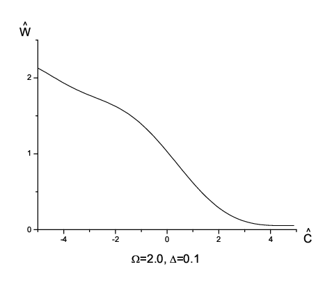
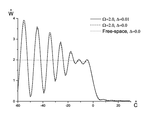
Another possibility is to set a certain value for and to plot the function for different values of . Since it does not make sense to consider values , because they are outside of the region of applicability of the resonance approximation. This explains the range of in Fig. 9 and Fig. 10. In particular we fixed and we plot the case for in Fig. 9 and values for and in Fig. 10. It is interesting to remark the characteristic behavior in Fig. 10, where one can distinguish peaks at certain values of . These peaks correspond to those values of such that . At these values, the -th TE or TM mode is at resonance. Contrast of peaks becomes better as increases, because different resonances are further away and peaks overlap less. For larger values of , as the number of excited modes increases, overlapping between different resonances hides the peaks, and one has the free-space limit (also shown for comparison in Fig. 10). Note that by definition of , the integrated power density is normalized to the angle-integrated power density in free-space at resonance, i.e. at . This explains why at in Fig. 10.


Finally, we may asses the influence of the waveguide on the output radiation by comparing the modulus of the vertical electric field for different values of with the modulus of the horizontally polarized field in free-space. In fact, as has been said before, the presence of boundary conditions different from those of free-space destroy the horizontal polarization as well as the azimuthal symmetry of the undulator radiation. Vertical and horizontal field are to be considered as functions of the distance from the axis. Since the modulus of the vertical electric field is not azimuthal symmetric we take a cut in the direction where it is maximal, i.e. at , as it can be seen inspecting Eq. (178). As done before we limit our analysis for exemplification purposes to the case . We are thus interested in the functions and respectively defined as
| (201) |
and
| (202) |
We studied as a function of for different values of and different values of . We set . Comparisons with (studied at ) as a function of at different values of are presented in Fig. 11 for , Fig. 12 for and Fig. 13 for at different values of . Note that the maximal value of is , and is due to the fact that the pipe poses a geometrical limit to the transverse region of interest. Figures underline the role of the vertical polarization component of the field for values of around unity. Thus, the level of the vertical polarization component of the field compared with that of the horizontal polarization gives a measure of the waveguide influence.

As it is clear by inspection of Eq. (160) and Eq. (161), our method allows straightforwardly to study the evolution of the radiation pulse after the undulator, provided that the pipe section remains unvaried. In Fig. 14 we show the evolution of the intensity profile as a function of the normalized distance from the center of the undulator . We take , and .
To conclude this Section we estimate the range of parameters of interest in the case of the infrared undulator beamline at FLASH. The wavelength range is between m and m. The radius of the vacuum pipe is cm, the number of undulator periods with a period length cm, yielding m. Note that the parameter is always much larger than unity, increasing when the wavelength is increased by ramping up the magnetic field in the undulator ( in the THz-gap operation range). This set of parameters means and . As it can be seen in Fig. 6 and 11, for in the short wavelength limit () the vacuum chamber has a small influence on the field distribution and polarization. A strong influence is visible, instead, in the long wavelength range (). Finally, from Fig. 8 we see that the total power at perfect resonance () is practically independent of the wavelength in our range of interest.
7 Wall-resistance effects
Up to now we studied the problem of undulator radiation in a waveguide assuming perfectly conducting walls, i.e. infinite conductivity . In this Section we follow the approach proposed in FELB to describe the case when the refractive index of the walls is still mainly defined by the conductivity (i.e. we are still dealing with a metal), but has a finite value. We will conclude that in practical situations of interest, the presence of wall-resistance effects introduce important changes to the theory for perfectly conductive walls.
Let us start our investigations with Maxwell’s equations in the time domain, written in all generality for a medium having conductivity and permittivity :
| (203) | |||
| (204) |
For a monochromatic wave of angular frequency we have
| (205) | |||
| (206) |
where
| (207) |
is the complex refractive index of the medium. A single equation for can be written as
| (208) |
A solution of Eq. (208) is a plane wave specified by:
| (209) | |||
| (210) |
where is the (complex) wave vector inside the metal, with a complex number.
Let us consider a plane wave at the interface between vacuum (with unitary refraction index) and a medium described by Eq. (207), and let be the wave vector of the incident wave in vacuum with . We indicate with subscripts and the tangential and normal components wave vectors to the metallic surface. Continuity of the tangential component of the wave vector on the boundary (i.e. ) implies:
| (211) |
As a result one obtains
| (212) |
In a metal, the refractive index is mainly defined by the conductivity according to
| (213) |
Since , also , and Eq. (212) yields
| (214) |
Thus, the propagation direction of the wave in the metal is almost perpendicular to the surface, independently of the direction of the incident wave. This means that electric and magnetic field into the metal have only tangential components, and . Moreover, these components must be continuous on the surface, as follows from Maxwell’s equations. Using Eq. (210) one obtains
| (215) |
Eq. (215) can be considered as an approximate boundary condition. Note that this is valid not only for plane waves. In fact, any wave can be decomposed in terms of a linear superposition of plane waves. Since Eq. (215) is valid for each component, it must be valid for their linear superposition. Eq. (215) can also be extended for any shape of the boundary surface, provided that typical value of the curvature radius is much larger than the wavelength. Eq. (215) is named after Leontovich, who first derived it, and can be written in vector form as
| (216) |
where the vector , as defined as in Section 3 and shown in Fig. 2, is pointing inwards. Using Leontovich boundary condition gives a good approximation in the case of a metallic waveguide, and drastically simplifies the solution of the electrodynamical problem. Namely, the problem of mode excitation in a waveguide with resistive walls can be solved following the same approach in Section 3 and Section 4, where boundary conditions are now substituted by Eq. (216).
Since we are applying the paraxial approximation, we assume that the field amplitude does not change much along the direction within a wavelength and we are interested about the (main) transverse components of the field and . Using Eq. (216) and Maxwell’s equations, Eq. (206), it is possible to find boundary conditions involving the transverse field components only.
| (217) |
The transverse components of Eq. (217) only involve , while the component along only involves . We may thus write
Second, from Eq. (216) we see that, on , the projections of and on the plane orthogonal to , i.e. and , are orthogonal and their modulus are related by Eq. (215). As a result, we have . Now, Eq. (206) implies . Therefore . But Eq. (206) also yields . We then obtain
| (219) |
If we now calculate the expression in brackets in Eq. (219) and we account for the fact that, in paraxial approximation, we can re-write Eq. (219) in terms of slowly varying field amplitudes as
| (220) |
that will substitute the second boundary condition in Eq. (51).
Thus, the problem in (51) should be substituted with
We may now follow the same method used in Section 3 to solve (7). Namely, after consistent application of Laplace transformations, we find an eigenvalue problem analogous to (59):
| (225) |
As for the case of perfectly metallic walls, boundary conditions are homogeneous, so that the domain of the Laplacian operator is the vector space of twice differentiable (square integrable) functions obeying boundary conditions in (225). However, the Laplacian operator defined in this way is not self-adjoint with respect to the inner product defined in Eq. (60). This is a result of the fact that vectors in Eq. (225), at the boundary, are not orthogonal to the surface . Then, eigenvalues are not real, nor eigenfunctions are orthogonal with respect to the inner product in Eq. (60). In general we do not know wether the spectrum is discrete, completeness is not granted and we cannot prove the existence of a set of eigenfunctions either. Yet, direct calculations in FELB show that
| (226) |
It follows that functions form a bi-orthogonal set of eigenfunctions. Bi-orthogonality is often exploited in different problems (see e.g. KRIB, SIEG, PLAS). In particular we will take advantage, without proving it, of completeness and discreteness of the bi-orthogonal set. This allows us to decompose as
| (227) |
exactly as for the case of perfectly conducting walls. Note that now eigenvalues and eigenfunctions are complex. In particular, we write the eigenvalues as
| (228) |
We want to study the problem of wall-resistance in the framework of a perturbation theory. If is an unperturbed eigenvalue (perfectly conductive walls) we require that for any value of .
In this case we may still formulate an eigenvalue problem for the two scalar (and complex) functions and with complex eigenvalues , using a definition analogous to Eq. (64). We get:
| (229) |
where
| (230) |
It should be noted that (229) is valid only within the framework of a perturbation theory. In fact, according to (229), functions separately obey Helmholtz’s equation, but boundary conditions in (229) are not consistent with independency of required by Eq. (64).
In the framework of a perturbation theory though, we may still use (229) and formally obtain the same tensor Green’s function in Eq. (78). As said above, we want to work in the framework of perturbation theory. We base such theory on the small parameter . Within this theory, the problem in (229) can be written as
| (235) |
where TE and TM modes are now decoupled. If we restrict our analysis to a circular waveguide radius , we obtain the following expression for at the first order in :
and
where should now be calculated with the help of Eq. (230), while boundary conditions in (235) allow to obtain
| (246) |
and
| (247) |
Note that Eq. (246) and Eq. (247) can be written in terms of our small parameter, since , where the concept of transverse wave number is now applied to each mode . Actually condition can be presented as and . Thus, we may give an estimation of wall resistance effects retaining our main results, Eq. (177) and Eq. (178), and substituting with and . In our case of interest, so that
| (248) |
and
| (249) |
Addition of and implies an exponential damping of each mode, due to the propagation factor in the expressions for , Eq. (179) and Eq. (180). We can estimate the damping exponent as
| (250) |
for TE modes, where we used and
| (251) |
for TM modes. Expressions for the damping exponents and , Eq. (250) and Eq. (251), are known in literature and may be found, for example, in LEWI. Note that the difference between and is only in the factor in Eq. (250). depends on the mode number, , while is independent of it.
Let us study a practical case for copper. We know that the skin depth for copper at wavelength cm is m and , where is the conductivity. It follows that for m, that is in the range of interest for the FLASH infrared beamline we obtain nm yielding
| (252) |
Let us consider cm and m (corresponding to ), and substitute these values in Eq. (250) and Eq. (251). The perturbation parameter is smaller than unity: (), and (). Therefore, we may apply the perturbation approach for estimations. It should be noted here that the accuracy of the first-order perturbation approach becomes better and better for higher modes, because and increase while increases. For the transverse magnetic modes we have a damping factor common to all modes . For transverse electric modes we should specify the mode number. For the first mode (), and we obtain . For second mode () we have and thus , that gives a negligible effect. All TM modes are visibly damped. At , i.e. half undulator length after the exit of the device, one has a damping factor , i.e. modes are dumped by about . TE modes instead, are left almost unaffected.
We conclude that propagation through the pipe is strongly affected by wall-resistance effects even for relatively large values of . Note that this effect strongly depends on the material considered. For example steel has a skin depth three times thicker than copper. Strictly speaking we could not apply a perturbation approach, since now the perturbation parameter is larger than unity (although comparable with unity). However, if we still use the perturbation approach to get a rough estimation, we obtain that TM modes present a dumping exponent that is about three times larger than copper. This means that TM modes are dumped by about . These estimations allow us to formulate the following recommendation: the internal part of the vacuum pipe for the infrared undulator line at FLASH should be copper-coated66 6 We underline the fact that these remarks are only valid in the case of undulator radiation. In particular, as said before, we will treat edge-radiation setups in a separate work..
8 Conclusions
In this article we presented the first exhaustive theory of undulator radiation within a waveguide and we exemplified it in the case of the infrared undulator beamline at FLASH. In the relatively simpler free-space case, paraxial Maxwell’s equations can be solved in terms of a scalar paraxial Green’s function. In that case, the solution for the field, written in reduced form within the resonance approximation is identical (aside for polarization properties) for planar and helical undulator configurations. When a waveguide is present, the relation between current sources and electromagnetic field is more complicated. The analysis of the problem is performed by introducing a tensor Green’s function technique, thus complicating the structure of equations that, in contrast to the free-space case, now depends on the undulator type and on the waveguide geometry. First we outlined a solution for a homogeneous waveguide with arbitrary cross-section. Then we specialized our consideration to the case of a circular waveguide, and we implemented the planar undulator case77 7 We treated the helical case in Appendix A. within the applicability region of the resonance approximation. The electric field was found as a superposition of the waveguide modes, and was studied for different values of parameters. The main parameter involved in the problem is the waveguide parameter , that can be interpreted as the squared ratio between the waveguide radius and the radiation diffraction size, and is a purely geometrical parameter. When is comparable, or smaller than unity, waveguide effects become important, under the assumption of a perfect conductor. Moreover, we found that wall-resistance effects play a significant role even for relatively large values of . To minimize this effect, it is desirable to coat the internal part of the waveguide with copper.
9 Acknowledgements
The authors are grateful to Martin Dohlus, Michael Gensch and Oliver Grimm (DESY) for many useful discussions and to Massimo Altarelli and Jochen Schneider (DESY) for their interest in this work.
Appendix A: Helical undulator
We define in all generality the horizontal and vertical velocity of an electron as a function of the longitudinal position along the undulator as
| (253) | |||
| (254) | |||
| (255) |
The sign in the second equation in (255) indicates an electron rotating clockwise ( sign) or counterclockwise ( sign) in the judgement of an observer located after the undulator and looking towards the device. The longitudinal Lorentz factor is now constant. We can write the phase factor in Eq. (80) as
| (256) |
The next step is to substitute Eq. (255) and Eq. (256) in Eq. (80) to calculate the field components. We can do that within the region of applicability of the resonance approximation, as in the case of a planar undulator. Within the region of applicability of the resonance approximation, condition (155), and neglecting negligible terms in Eq. (80) as specified in Section 5 we obtain the field components in cartesian coordinates for the case of a helical undulator:
| (257) |
By inspection of Eq. (4), under the resonance approximation only the terms with survive. With the help of Eq. (4) and neglecting negligible terms we find for the horizontal field () and for the vertical field () respectively:
| (258) | |||||
| (259) |
and
| (260) | |||||
| (261) |
One can also write the expressions for the components in polar coordinates and , that are related to and through
We thus obtain
| (265) | |||||
| (266) |
and
| (267) | |||||
| (268) |
Note that both TM and TE modes are present in the expression for the field. It is interesting to compare this fact with what can be found in literature. As already remarked in Section 1, TM modes are neglected in HART. For the readers’ commodity we report here words from Section 9.3 of reference HART. There one may find: ”It is easily seen that in the case of a spatially extended charge propagating in a helical wiggler, the TE modes (…) couple to the wiggler-induced motion, as the current components (…) By contrast, the TM modes (…) are driven by the uniform motion of the space-charge distribution in the cylindrical waveguide. Therefore, in the remainder of this derivation, we will focus on the TE modes”.
Neglecting TM modes is held by us as a misconception. If it was correct, also undulator radiation produced by planar undulators should exhibit only TE modes. In fact, as already discussed in Section 5, the field from a planar undulator can be seen as superposition of fields from two helical trajectories. Without TM modes we could not even recover the free-space limit for as studied in Section 5 for a planar undulator. In particular, we would loose both horizontal polarization and azimuthal symmetry of the field.
Similarly, one can study the limit for the helical case, following a procedure analogous to that in Section 5 for a planar undulator. In analogy with the planar case, one can show that if TM modes are neglected, both circular polarization and azimuthal symmetry of the field are lost.
Neglecting TM modes in HART is the result of a more general misconception introduced when Maxwell’s equations are solved with the Green’s function approach. Namely, the misconception is introduced in the eigenmode decomposition of the four-current (see paragraph 5.6.4 of HART), where TM modes are not coupled with the transverse current density as they must be.
References
- [1] H. Wabnitz et al., Nature, 420, 482-485 (2002)
- [2] L. Juha et al. Nucl. Instrum. Meth. Phys. Res. A, 507, 577-581 (2003)
- [3] V. Ayvazyan et al., Phys. Rev. Lett, 88, 104802 (2002)
- [4] V. Ayvazyan et al., Eur. Phys. J. D, 20, 149-156 (2002)
- [5] V. Ayvazyan et al., Eur. Phys. J. D, 37, 297-303 (2006)
- [6] G. Gehrke and J. Feldhaus, Synch. Rad. News, 19, 20-24 (2006)
- [7] B. Faatz et al, Nucl. Instrum. Meth. Phys. Res A, 475, 363-367 (2001)
- [8] G. Geloni, E. Saldin, E. Schneidmiller and M. Yurkov, Nucl. Instrum. Meth. Phys. Res. A, 528, 184-188 (2004)
- [9] G. Geloni, E. Saldin, E. Schneidmiller and M. Yurkov, Nucl. Instrum. Meth. Phys. Res. A, 528, 330-334 (2004)
- [10] O. Grimm, P. Schmueser, ”Principles of longitudinal beam diagnostics with coherent radiation”, TESLA-FEL 2006-03 (2006)
- [11] V. Borisov et al., in Proc. of the 10th European Particle Accelerator Conference EPAC’06, Edinburgh, UK, 2595-2595 (2006)
- [12] O. Grimm, private communication
- [13] M. Gensch, private communication
- [14] O. Chubar and P. Elleaume, in Proc. of the 6th European Particle Accelerator Conference EPAC’98, Stockholm, Sweden, 1177-1179 (1998)
- [15] T. Tanaka and H. Kitamura, J. Synch. Rad. 8, 1221 (2001)
- [16] G. Geloni, E. Saldin, E. Schneidmiller and M. Yurkov, ”Fourier Optics Treatment of Classical Relativistic Electrodynamics”, DESY 06-127 (2006)
- [17] H. Motz and M. Nakamura, Ann. Phys. 7, 84 (1959)
- [18] H.A. Haus and N. Islam, J. Appl. Phys. 54, 9 (1983)
- [19] A. Amir, I. Boscolo and L. R. Elias, Phys. Rev A, 32, 5 (1985)
- [20] F.V. Hartemann, ”High Field Electrodynamics”, CRC Press (2002)
- [21] E. Saldin, E. Schneidmiller and M. Yurkov, ”The Physics of Free Electron Lasers”, Springer, Berlin, 2000, ISBN 3-540-66266-9
- [22] ZEMAX code, at http://www.zemax.com/
- [23] G. Geloni, E. Saldin, E. Schneidmiller and M. Yurkov, Opt. Comm., 271, 1, 207 (2007)
- [24] B. Kinkcaid, J. Appl. Phys, 48, 7, 2684 (1977)
- [25] D. Alferov, Y. Bashmakov and E. Bessonov, Sov. phys. - Tech. Phys. 18, 1336 (1974)
- [26] H. Wiedemann, Particle accelerator physics, Springer-Verlag (1993)
- [27] A. Gover, Phys. Rev. ST Accel. Beams 8, 030701 (2005)
- [28] A. Gover, Phys. Rev. ST Accel. Beams 8, 030702 (2005)
- [29] S. Krinsky, IEEE Trans. Nucl. Sci. 30, 3078 (1983); G. K. Green, Brookhaven National Laboratory Report No. 50522 (1976)
- [30] S. Krinsky and L.H. Yu. Phys. Rev. A 35, 3406 (1987)
- [31] A.E. Siegman, Phys. Rev. A 39, 1253 (1989)
- [32] G. Geloni, E. Saldin, E. Schneidmiller and M. Yurkov, Nucl. Instrum. Meth. Phys. Res. A, 554, 1, 20 (2005)
- [33] L. Lewin, ”Theory of waveguides”, London, Newnes-Butterworths and Co. (1975)