Self-Organized Network Flows
Abstract
A model for traffic flow in street networks or material flows in supply networks is presented, that takes into account the conservation of cars or materials and other significant features of traffic flows such as jam formation, spillovers, and load-dependent transportation times. Furthermore, conflicts or coordination problems of intersecting or merging flows are considered as well. Making assumptions regarding the permeability of the intersection as a function of the conflicting flows and the queue lengths, we find self-organized oscillations in the flows similar to the operation of traffic lights.
keywords
Traffic flows, production, emergent oscillations, self-organized traffic lights, synchronizationDirk Helbing,1,2 Jan Siegmeier,1 and Stefan Lämmer1
1 Institute for Transport & Economics, Dresden University of Technology
Andreas-Schubert-Str. 23, 01062 Dresden, Germany
2 Collegium Budapest – Institute for Advance Study
Szentháromság utca 2, 1014 Budapest, Hungary
(Communicated by Aim Sciences)
1 Introduction
Material flows are found in many places of the world. This concerns, for example, traffic flows in urban areas or flows of commodities in logistic systems. There is also some similarity with material flows in production or biological systems, from cells over bodies upto ecological food chains. Many of these material flows are not of diffusive nature or going on in continuous space. They are often directed and organized in networks. In comparison with data flows in information networks, however, there are conservation laws, which can be used to set up equations for material flows in networks. It turns out, however, that this is not a trivial task. While there is already a controversial discussion about the correct equations representing traffic flows along road sections [6, 11, 33, 26], their combination in often complex and irregular networks poses further challenges. In particular, there have been several publications on the treatment of the boundary conditions at nodes (connections) of several network links (i.e. road sections) [25, 7, 28, 14, 10, 9, 4, 22, 23, 24]. In particular, the modelling of merging and intersecting flows is not unique, as there are many possible forms of organization, including the use of traffic lights. Then, however, the question comes up how these traffic lights should be operated, coordinated, and optimized. In order to address these questions, in Sec. 2 we formulate a simple model for network flows, which contains the main ingredients of material or traffic flows. Section 3 will then discuss the treatment of diverges, merges, and intersections. Equations for the interaction-dependent permeability at merging zones and intersections will be formulated in Sec. 4. We will see that, under certain conditions, they lead to spontaneous oscillations, which have features similar to the operation of traffic lights. Finally, Sec. 5 summarizes and concludes this paper.
2 Flows in Networks
The following section will start with a summary of the equations derived for traffic flows in networks in a previous paper. These equations are based on the following assumptions:
- •
The road network can be decomposed into road sections of homogeneous capacity (links) and nodes describing their connections.
- •
The traffic dynamics along the links is sufficiently well described by the Lighthill-Whitham model, i.e. the continuity equation for vehicle conservation and a flow-density relationship (“fundamental diagram”). This assumes adiabatic speed adjustments, i.e. that acceleration and deceleration times can be neglected.
- •
The parameters of vehicles such as the maximum speed and the safe time headway are assumed to be identical in the same road section, and who enters a road section first exits first (FIFO principle). That is, overtaking is assumed to be negligible.
- •
The fundamental diagram can be well approximated by a triangular shape, with an increasing slope at low densities and a decreasing slope in the congested regime. This implies two constant characteristic speeds: While corresponds to the free speed or speed limit on road section ,
(1) the dissolution speed of the downstream front of a traffic jam and the velocity of upstream propagation of perturbations in congested traffic. While denotes the maximum vehicle density in vehicle queues, s is the safe time gap between two successive vehicles.
- •
The vehicle density in traffic jams is basically constant.
These assumptions may be compensated for by suitable corrections [11], but already the model below displays a rich spectrum of spatio-temporal behaviors and contains the main elements of traffic dynamics we are interested in here.
2.1 Flow Conservation Laws
In the following, we will introduce our equations for traffic flows in networks very shortly, as a detailed justification and derivation has been given elsewhere [12, 13, 14]. These equations are also meaningful for pipeline networks [3] (if complemented by equations for momentum conservation), logistic systems [21], or supply networks [19]. Our notation is illustrated in Fig. 1.
Compared to Ref. [14], we will use a simplified notation, here.11 1 The arrival flow has previously been denoted by , the potential arrival flow by , the departure flow by and the potential departure flow by . The arrival flow denotes the actual inflow of vehicles into the upstream end of road section , while is the actual departure flow, i.e. the flow of vehicles leaving road section at its downstream end. The quantity
| (2) |
represents the maximum in- or outflow of road section . All the above quantities refer to flows per lane. is the number of lanes and the length of road section . is the length of the congested area on link (measured from the downstream end), and is the number of stopped or delayed vehicles, see Eqs. (16) and (14). With these definitions, we can formulate constraints for the actual arrival and departure flows, which are given by the potential arrival flows and the potential departure flows , respectively.
The actual arrival flow is limited by the maximum inflow , if road section is not fully congested (). Otherwise (if ) it is limited by the actual departure flow a time period before, as it requires this time period until the downstream flow value has propagated upto the upstream end of the road section by forward movement of vehicles under congested traffic conditions. This implies
| (3) |
Moreover, the potential departure flow of road section is given by its permeability times the maximum outflow from this road section, if vehicles are queued up () and waiting to leave. Otherwise (if ) the outflow is limited by the permeability times the arrival flow a time period before, as this is the time period that entering vehicles need to reach the end of road section when moving freely at the speed . This gives the additional relationship
| (4) |
The permeability for traffic flows at the downstream end of section can assume values between 0 and 1. In case of a traffic light, corresponds to a green light for road section , while corresponds to a red or amber light.
Alternatively and shorter than Eqs. (3) and (4) one can write
| (5) |
and
| (6) |
where the Heaviside function is 1, if the argument (inequality) has the logical value “true”, otherwise it is 0. Note that the above treatment of the traffic flow in a road section requires the specification of the boundary conditions only, as we have integrated up Lighthill’s and Whitham’s partial differential equation over the length of the road section. The dynamics in the inner part of the section can be easily reconstructed from the boundary conditions thanks to the constant characteristic speeds. However, a certain point of the road section may be determined either from the upstream boundary (in the case of free traffic) or by the downstream boundary (if lying in the congested area, i.e. behind the upstream congestion front). Therefore, we have a switching between the influence of the upstream and the downstream boundary conditions, which makes the dynamics both, complicated and interesting. This switching results from the maximum functions above and implies also that material flows in networks are described by hybrid equations. Although the dynamics is determined by linear ordinary differential equations in all regimes, the switching between the regimes can imply a complex dynamics and even deterministic chaos [32].
Complementary to the above equations, we have now to specify the constraints for the nodes, i.e. the connection, merging, diverging or intersection points of the homogeneous road sections. Let the ingoing links be denoted by the index and the outgoing ones by . To distinguish quantities more easily when we insert concrete values for and , we mark quantities of outgoing links additionally by a prime (′).
Due to the condition of flow conservation, the arrival flow into a road section with lanes must agree with the sum of the fractions of all outflows turning into road section . Additionally, the arrival flows are limited, i.e. we have
| (7) |
for all . Of course, the turning fractions are normalized due to flow conservation:
| (8) |
In cases of no merging flows, Eq. (7) simplifies to
| (9) |
for all . At the same time, must be fulfilled for all . Together, this implies
| (10) |
for all .
The advantage of the above model is that it contains the most important elements of the traffic dynamics in networks. This includes the transition from free to congested traffic flows due to lack of capacity, the propagation speeds of vehicles and congested traffic, spillover effects (i.e. obstructions when entering fully congested road sections) and, implicitly, load-dependent travel times as well.
2.2 Two Views on Traffic Jams
Let us study the traffic dynamics on the road sections in more detail. Traffic jams can be handled in two different ways: First by determining the number of cars that are delayed compared to free traffic or, second, by determining fronts and ends of traffic jams. The former method is more simple, but it cannot deal correctly with spill-over effects, when the end of a traffic jam reaches the end of a road section. Therefore, the first method is sufficient only in situations where the spatial capacity of road sections is never exceeded.
2.2.1 Method 1: Number of Delayed Vehicles
The first method just determines the difference between the number of vehicles that would reach the end of road section upto time and the number of vehicles that actually leave the road section upto this time. just corresponds to the number of vehicles which have entered the road section upto time , as is the free travel time. This implies
| (11) |
while the number of vehicles that have acually left the road section upto time is
| (12) |
Hence, the number of delayed vehicles is given by
| (13) |
Alternatively, one can use the following differential equation for the temporal change in the number of delayed vehicles:
| (14) |
In contrast, the number of all vehicles on road section (independently of whether they are delayed or not) changes in time according to
| (15) |
2.2.2 Method 2: Jam Formation and Resolution
In our simple macroscopic traffic model, the formation and resolution of traffic jams is described by the shock wave equations, where we have the two characteristic speeds (the free speed) and (the jam resolution speed). According to the theory of shock waves [29, 37], the upstream end of a traffic jam, which is located at a place upstream of the end of road section , is moving at the speed
| (16) |
with the (free) density
| (17) |
immediately before the upstream shock front and the (congested) density
| (18) |
immediately downstream of it. This is, because free traffic is upstream of the shock front, and congested traffic downstream of it (for details see Eqs. (1.6) and (1.4) in Ref. [14]). In contrast, the downstream front of a traffic jam is moving at the speed
| (19) |
since congested traffic with zero flow is upstream of the shock front and free traffic flow occurs downstream of it.
2.2.3 Comparison of the Two Methods
Let us discuss a simple example to make the differences of both descriptions clearer. For this, we assume that, at time , traffic flow on the overall road section is free, i.e. any traffic jam has resolved and there are no delayed vehicles. The flow shall be stopped by a red traffic light for a time period . At time , the traffic light shall turn green, and the formed traffic jam shall resolve. For the arrival flow, we simply assume a constant value , and the road section shall be long enough to take up the forming traffic jam. Moreover, the departure flow shall be . Then, according to method 1, the number of delayed vehicles at time is
| (20) |
and it is reduced according to
| (21) |
Therefore, any delays are resolved after a time period
| (22) |
i.e. at time
| (23) |
Afterwards, .
In contrast, the end of the traffic jam grows with the speed
| (24) |
Therefore, we have . Surprisingly, this is greater than , i.e. the expected length of the traffic jam based on the number of delayed vehicles. The reason is that the delay of a vehicle joining the traffic jam at location is noticed at the downstream end of the road section only after a time period .
The resolution of the traffic jam starts from the downstream end with the speed
| (25) |
if the outflow is free (i.e. ), otherwise with the speed
| (26) |
since congested traffic with zero flow and maximum density is upstream of the shock front.
Obviously, the jam resolution has reached the further growing, upstream jam front when . Therefore, the jam of density has disappeared after a time period , i.e. at time
| (27) |
Surprisingly, it can be shown that , i.e. the traffic jam resolves before the number of delayed vehicles reaches a value of zero. In fact, it still takes the time until the last delayed vehicle has left the road section, where
| (28) |
is the shock front between free upstream traffic flow and the congested outflow , which usually differs from the speed of outflowing vehicles. For , we have because of .
Undelayed traffic starts when this shock front reaches the end of the road section, i.e. at time
| (29) |
Inserting eventually gives . This agrees perfectly with the above result for the first method (based on vehicle delays rather than traffic jams).
In conclusion, both methods of dealing with traffic jams are consistent, and delayed vehicles occur as soon as traffic jam formation begins. However, according to method 1, a queued vehicle at position is counted as delayed only after an extra time period , but it is counted as undelayed after the same extra time period. This is because method 1 counts on the basis of vehicle arrivals at the downstream end of road section .
As it is much simpler to use the method 1 based on determining the number of delayed vehicles than using method 2 based on determining the movement of shock fronts, we will use method 1 in the following. More specifically, in Eq. (3) we will replace by and by . This corresponds to a situation in which the vehicles would not queue up along the road section, but at the downstream end of the road section, like in a wide parking lot or on top of each other. As long as road section is not fully congested, this difference does not matter significantly. If it is fully congested, the dynamics will potentially be different, defining a modified model of material network flows. However both, the original and the modified model fulfill the conservation equation and show spillover effects.
2.2.4 Calculation of Cumulative and Maximum Individual Waiting Times
In Ref. [12], we have derived a delay differential equation to determine the travel time of a vehicle entering road section at time (see also Ref. [1, 2, 5]):
| (30) |
According to this, the travel time increases with time, when the arrival rate at the time of entry exceeds the departure rate at the leaving time , while it decreases when it is lower. It is remarkable that this formula does not explicitly depend on the velocities on the road section, but only on the arrival and departure rates.
Another method to determine the travel times is to integrate up over the number of vehicles arriving in road section ,
| (31) |
and over the number of vehicles leaving it,
| (32) |
starting at at time when there are no vehicles in the road. If denotes the time at which , then is the travel time of a vehicle entering road section at time and
| (33) |
is its waiting time.
Another interesting quantity is the cumulative waiting time , which is determined by integrating up over the number of all delayed vehicles. We obtain
| (34) | |||||
and the differential equation
| (35) |
For a constant arrival flow and a red traffic light from to (i.e. ), we find
| (36) |
In this time period, a number of vehicles accumulates, which gives an average waiting time of
| (37) |
at the end of the red light. The first vehicle has to wait twice as long, namely, a time period .
3 Treatment of Merging, Diverging and Intersection Points
While the last section has given general formulas that must be fulfilled at nodes connecting two or more different links, in the following we will give some concrete examples, how to deal with standard elements of street networks. For previous treatments of traffic flows at intersections see, for example, Refs. [9, 25, 7, 28].

3.1 Diverging Flows: One Inflow and Several Outflows
3.2 Merging Flows: Two Inflows and One Outflow
We assume a flow that splits into two flows (going straight) and (turning right), but a right-turning flow merging with flow , as in turn-right-on-red setups (see Fig. 1b). For this situation, we have the equations
| (42) | |||||
| (43) |
One can derive
| (44) |
and
| (45) |
Let us set
| (46) |
and
| (47) |
Then, it can be shown that and , as demanded. If is chosen a value smaller than specified in Eq. (46), but is still set to the maximum related value according to Eq. (47), the overall flow
| (48) |
is reduced as long as , since this goes along with additional turning flows (while the number of lanes does not matter!). Therefore, it is optimal to give priority to the outflow according to Eq. (46) and to add as much outflow as capacity allows. This requires suitable flow control measures, otherwise the optimum value of the overall flow could not be reached. In fact, the merging flow would “steel” some of the capacity reserved for the “main” flow (), which would reduce the possible outflow and potentially cause a breakdown of free traffic flow, as it is known from on-ramp areas of freeways [34] .
3.3 A Side Road Merging with a Main Road
Compared to the last section, the situation simplifies, if we have just a side road or secondary turning flow merging with a the flow of a main road without any turning flow away from the main road. In this case, we have and , which leaves us with the relationships
| (49) |
and
| (50) |
3.4 Intersection-Free Designs of Road Networks
With the formulas for the treatment of merges and diverges in the previous sections, it is already possible to simulate intersection-free designs of urban road networks, which do not need any traffic light control. The most well-known design of intersection-free nodes are roundabouts (see the upper left illustration in Fig. 2). It is, however, also possible to construct other intersection-free designs based on subsequent merges and diverges of flows with different destinations. Two examples are presented in Fig. 2b and c.


Although intersection-free designs require the driver to take small detours, such a road network will normally save travel time and fuel, given that the traffic volume is not too low. This is because intersections then need to be signalized in order to be safe and efficient.22 2 Of course, a first-come-first-serve or right-before-left rule will be sufficient at small traffic volumes. Traffic signals, however, imply that vehicles will often be stopped for considerable time intervals. This causes significant delays, at least for vehicles not being served by a green wave. Intersection-free designs, in contrast, do not necessarily require vehicles to stop. Therefore, the average speeds are expected to be higher and the travel times lower than for road networks with intersections. This has significant implications for urban transport planning, if intersections cannot be avoided by bridges or tunnels.
3.5 Two Inflows and Two Outflows
The treatment of intersecting flows is more complicated than the treatment of merges and diverges. Moreover, the resulting flows are only uniquely defined, if additional rules are introduced such as the optimization of the overall flow. Let us here treat the case of an intersection with two inflows and two outflows (see Fig. 1c). Equation (5) implies the inequalities
| (51) |
with the constraints
| (52) |
so that is automatically fulfilled. The constraints (52) define an rectangular area of possible -values in the - plane, where the size of the rectangle varies due to the time-dependence of . The inequalities (51) can be rewritten as
| (53) |
and
| (54) |
They potentially cut away parts of this rectangle, and the remaining part defines the convex set of feasible points at time . We are interested to identify the “optimal” solution , which maximizes the overall flow
| (55) |
As this defines a linear optimization problem, the optimal solution corresponds to one of the corners of the convex set of feasible points, namely the one which is touched first by the line
| (56) |
when we reduce from high to low values.
Let us, therefore, determine all possible corners of the convex set and the conditions, under which they correspond to the optimal solution. We will distinguish the following cases:
- (a)
None of the boundary lines (53) and (54) corresponding to the equality signs cuts the rectangle defined by and in more than 1 point. This case applies, if and , as and implies that both lines are falling or at least not increasing. Since the line (56) reflecting the goal function is falling as well, the optimal point is
(57) i.e. the outer corner of the rectangle corresponding to the potential or maximum possible departure flows (see Fig. 3).
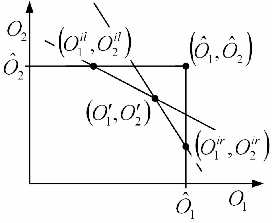
Figure 3: Illustration of the possible optimal solutions for two intersecting flows (see text for details). - (b)
Only one of the two boundary lines/border lines, or , cuts the rectangle in more than one point. Let us assume, this holds for line , i.e. . Then, the left cutting point
(58) is the optimal point if , i.e. if the slope of the goal function (56) is smaller than the one of the cutting border line. Otherwise, if , the optimal point is given by the right cutting point
(59) (see Fig. 3).
- (c)
If both border lines cut through the rectangle, but one of them lies above the other line, then only the lower line determines the optimal solution, which can be obtained as in case (b). Case (c) occurs if and (line 1 is the lower one) or if and (line 2 is the lower one).
- (d)
The boundary lines cut each other in the inner part of the rectangle. This occurs if and . Then, the left-most cutting point is the optimal solution, if the slope of the goal function is smaller than the smallest slope of the two boundary lines, while it is the lower right cutting point , if is greater than the steepest slope of the two boundary lines, otherwise, the cutting point of the two boundary lines,
(60) is the optimal point (see Fig. 3). Mathematically speaking, we have
(61)
It is astonishing that the simple problem of two intersecting traffic flows has so many different optimal solutions, which sensitively depend on the parameter values. This can reach from situations where both outgoing road sections experience the maximum possible outflows upto situations, where the outflow in the system-optimal point becomes zero for one of the road sections. A transition from one optimal solution to another one could easily be triggered by changes in the turning fractions entering the parameters and , for example due to time-dependent turning fractions .
3.6 Inefficiencies due to Coordination Problems
An interesting question is how to actually establish the flows corresponding to the system optima that were determined in the previous sections on merging and intersecting flows. Of course, zero flows can be enforced by a red traffic light, while maximum possible flows can be established by a node design giving the right of way to one road (the “main” road). However, it is not so easy to support an optimimum point corresponding to mixed flows, such as . That would need quite tricky intersection designs or the implementation of an intelligent transportation system ensuring optimal gap usage, e.g. based on intervehicle communication. Only in special cases, the task could be performed by a suitable traffic light control.
In normal merging or intersection situations, there will always be coordination problems [16] when entering or crossing another flow, if the traffic volumes reach a certain level. This will cause inefficiencies in the usage of available road capacity, i.e. mixed flows will not be able to use the full capacity. Such effects can be modelled by specifying the corresponding permeabilities as a function of the merging flows, particularly the main flow or crossing flow. The deviation of from 1 will then be a measure for the inefficiency. A particularly simple, phenomenological specification would be
| (62) |
where the own outflow supports a high permeability and the intersecting outflow suppresses it. However, rather than using such a phenomenological approach, the permeability could also be calculated analytically, based on a model of gap statistics, since large enough vehicle gaps are needed to join or cross a flow. Such kinds of calculations have been carried out in Refs. [15, 30, 35, 36].
4 Towards a Self-Organized Traffic Light Control
In Ref. [14], it has been pointed out that, for not too small arrival flows, an oscillatory service at intersections reaches higher intersection capacities and potentially shorter waiting times than a first-in-first-out service of arriving vehicles. This is due to the fact that the outflow of queued vehicles is more efficient than waiting for the arrival of other freely flowing vehicles, which have larger time gaps. For similar reasons, pedestrians are passing a bottleneck in an oscillatory way [20], and also two intersecting flows tend to organize themselves in an oscillatory way [15, 17].
Therefore, using traffic lights at intersections is natural and useful, if operated in the right way. However, how to switch the traffic lights optimally? While this is a solvable problem for single traffic lights, the optimal coordination of many traffic lights [31] is a really hard (actually NP hard) problem [8]. Rather than solving a combinatorial optimization problem, here, we want to suggest a novel approach, which needs further elaboration in the future. The idea is to let the network flows self-organize themselves, based on suitable equations for the permeabilities as a function of the outflows and the numbers of delayed vehicles.
Here, we will study the specification
| (63) |
and
| (64) |
which generalizes formula (62). While the relative queue length
| (65) |
quantifies the pressure to increase the permeability for road section 1, the outflow from the road section 2 resists this tendency, while the flow on road section 1 supports the permeability. The increasing pressure eventually changes the resistance threshold and the service priority. An analogous situation applies to the permeability for road section 2, where the pressure corresponds to , which is again the difference in queue length. , , and are non-negative parameters. may be set to 1, while must be large enough to establish a sharp switching. Here, we have assumed . The parameter allows to influence the switching frequency , which is approximately proportional to . We have adjusted the frequency to the cycle time
| (66) |
which results if the switching (setup) time (“yellow traffic light”) is s and a green light is terminated immediately after a queue has dissolved after lifting the red light.33 3 If and denote the green time periods for the intersecting flows 1 and 2, respectively, the corresponding red time periods for a periodic signal control are and , to which the switching setup time of duration must be added. From formula (23) and with we obtain and . Using the definition for the cycle time, we finally arrive at Eq. (66). The corresponding parameter value is
| (67) |
Figure 4 shows a simulation result for and .

The properties of the corresponding specification of the permeabilitities are as follows:
- •
is non-negative and does not exceed the value 1.
- •
For the sum of permeabilities and , we have
(68) where we have introduced the abbreviation
(69) The sum is close to 1 for large absolute values of , while for the overall permeability is small.
- •
- •
With the specification (67) of parameter , the cycle time is approximately proportional to the overall inflow .
- •
The road section with the higher flow gets a longer green time period (see Fig. 4).
If the above self-organized traffic flows shall be transfered to a new principle of traffic light control, phases with could be interpreted as green phases and phases with as red phases. Inefficient, intermediate switching time periods for certain choices of parameter values could be translated into periods of a yellow traffic light.
5 Summary and Outlook
We have presented a simple model for conserved flows in networks. Although our specification has been illustrated for traffic flows in urban areas, similar models are useful for logistic and production system or even transport in biological cells or bodies. Our model considers propagation speeds of entities and congestion fronts, spill-over effects, and load-dependent transportation times.
We have also formulated constraints for network nodes. These constraints contain several minimum and maximum functions, which implies a multitude of possible cases even for relatively simple intersections. It turns out that the arrival and departure flows of diverges have uniquely defined values, while merges or intersections have a set of feasible solutions. This means, the actual result may sensitively depend on the intersection design. For mathematical reasons, we have determined flow-optimizing solutions for two merging and two intersecting flows. However, it is questionable whether these solutions can be established in reality without the implementation of intelligent transport systems facilitating optimal gap usage: In many situations, coordination problems between vehicles in merging or intersection areas cause inefficiencies, which reduce their permeability.
In fact, at not too small traffic volumes, it is better to have an oscillation between minimum and maximum permeability values. Therefore, we have been looking for a mechanism producing emergent oscillations between high and low values. According to our proposed specification (which is certainly only one of many possible ones), the transition between high and low permeability was triggered, when the difference between the queue lengths of two traffic flows competing for the intersection capacity exceeded a certain value. The resulting oscillatory service could be used to define traffic phases. One potential advantage of such an approach would be that the corresponding traffic light control would be based on the self-organized dynamics of the system. Further work in this direction seems very promising.
Acknowledgements
The authors are grateful for partial financial support by the German Research Foundation (research projects He 2789/5-1, 8-1) and by the “Cooperative Center for Communication Networks Data Analysis”, a NAP project sponsored by the Hungarian National Office of Research and Technology under grant No. KCKHA005.
References
- [1] V. Astarita, Flow propagation description in dynamic network loading models, in Y. J. Stephanedes and F. Filippi (eds.), Proc. IV Internat. Conf. Appl. Adv. Tech. Transportation Engrg (AATT), 1995, pp. 599–603.
- [2] V. Astarita, Node and link models for traffic simulation, Math. Comput. Model., 35 (2002), no. 5, 643–656.
- [3] M. K. Banda, M. Herty and A. Klar, Gas flow in pipeline networks, NHM, 1 (2006), no. 1, 41–56.
- [4] G. Bretti, R. Natalini and B. Piccoli, Numerical approximations of a traffic flow model on networks, NHM, 1 (2006), no. 1, 57–84 .
- [5] M. Carey, Y.E. Ge and M. McCartney, A whole-link travel-time model with desirable properties, Transport. Sci., 37 (2003), no. 1, 83–96.
- [6] C. F. Daganzo, Requiem for second-order fluid approximations of traffic flow, Transpn. Res. B, 29 (1995), 277–286.
- [7] C. F. Daganzo, The cell transmission model, Part II: Network traffic, Transpn. Res. B, 29 (1995), 79–93.
- [8] B. De Schutter, Optimizing acyclic traffic signal switching sequences through an extended linear complementarity problem formulation, Eur. J. Oper. Res., 139 (2002), no. 2, 400–415.
- [9] M. Garavello and B. Piccoli, Traffic Flow on Networks, American Institute of Mathematical Sciences, Springfield, 2006.
- [10] S. Goettlich, M. Herty and A. Klar, Modelling and optimization of supply chains on complex networks, Commun. Math. Sci., 4 (2006), no. 2, 315–330.
- [11] D. Helbing, Traffic and related self-driven many-particle systems, Rev. Mod. Phys., 73 (2001), 1067–1141.
- [12] D. Helbing, A section-based queueing-theoretical traffic model for congestion and travel time analysis in networks, J. Phys. Math. Gen. 36 (2003), L593–L598.
- [13] D. Helbing, Production, supply, and traffic systems: A unified description, in S. P. Hoogendoorn, S. Luding, P. H. L. Bovy, M. Schreckenberg and D. E. Wolf (eds.), Traffic and Granular Flow ’03, Springer, Berlin, 2005, pp. 173–188.
- [14] D. Helbing, S. Lämmer and J.-P. Lebacque, Self-organized control of irregular or perturbed network traffic, in C. Deissenberg and R. F. Hartl (eds.), Optimal Control and Dynamic Games, Springer, Dordrecht, 2005, pp. 239–274.
- [15] D. Helbing, R. Jiang and M. Treiber, Analytical investigation of oscillations in intersecting flows of pedestrian and vehicle traffic, Phys. Rev. E, 72 (2005), 046130.
- [16] D. Helbing, A. Johansson, J. Mathiesen, M. H. Jensen and A. Hansen, Analytical approach to continuous and intermittent bottleneck flows, Phys. Rev. Lett., 97 (2006), 168001.
- [17] D. Helbing, L. Buzna, A. Johansson, and T. Werner, Self-organized pedestrian crowd dynamics: Experiments, simulations, and design solutions, Transpn. Science, 39 (2005), 1–24.
- [18] D. Helbing and S. Lämmer, Method for the coordination of competing processes or for the control of the transport of mobile entities within a network, Patent DE 10 2005 023 742.8.
- [19] D. Helbing, S. Lämmer, T. Seidel, P. Seba and T. Platkowski, Physics, stability and dynamics of supply networks, Phys. Rev. E, 70 (2004), 066116.
- [20] D. Helbing and P. Molnár, Social force model for pedestrian dynamics, Phys. Rev. E, 51 (1995), 4282–4286.
- [21] D. Helbing, T. Seidel, S. Lämmer and K. Peters, Self-organization principles in supply networks and production systems, in: B. K. Chakrabarti, A. Chakraborti, and A. Chatterjee (eds.) Econophysics and Sociophysics, Wiley, New York, 2006.
- [22] M. Herty and A. Klar, Modeling, simulation, and optimization of traffic flow networks, SIAM Appl. Math., 64 (2003), no. 2, 565–582.
- [23] M. Herty and A. Klar, Simplified dynamics and optimization of large scale traffic flow networks Math. Mod. Meth. Appl. Sci., 14 (2004), no. 4, 579–601.
- [24] M. Herty, S. Moutari and M. Rascle, Optimization criteria for modelling intersections of vehicular traffic flow, NHM, 1 (2006), no. 2, 275–294.
- [25] M. Hilliges and W. Weidlich, A phenomenological model for dynamic traffic flow in networks, Transpn. Res. B, 29 (1995), 407–431.
- [26] B. Kerner, The Physics of Traffic, Springer, Berlin, 2004.
- [27] S. Lämmer, H. Kori, K. Peters and D. Helbing, Decentralised control of material or traffic flows in networks using phase-synchronisation, Phys. Stat. Mech. Appl., 363 (2006), 39–47.
- [28] J.-P. Lebacque and M. M. Khoshyaran, First-order macroscopic traffic flow models: Intersection modeling, network modeling, in H. S. Mahmasani (ed.), 16th International Symposium on Transportation and Traffic Theory, Elsevier, 2005, pp. 365-386.
- [29] M. J. Lighthill and G. B. Whitham, On kinematic waves: II. A theory of traffic on long crowded roads, Proc. Roy. Soc. London, Ser. A, 229 (1955), 317–345.
- [30] A. J. Mayne, Some further results in the theory of pedestrians and road traffic, Biometrika 41 (1954), pp. 375–389.
- [31] C. H. Papadimitriou and J. N. Tsitsiklis, The complexity of optimal queuing network control, Math. Oper. Res., 24 (1999), no. 2, pp. 293–305.
- [32] K. Peters and U. Parlitz, Hybrid systems forming strange billiards, Int. J. Bifurcation and Chaos, 13 (2003), no. 9, 2575–2588.
- [33] M. Schönhof and D. Helbing, Empirical features of congested traffic states and their implications for traffic modelling, Transpn. Sci, accepted (2006).
- [34] M. Treiber, A. Hennecke and D. Helbing, Congested traffic states in empirical observations and microscopic simulations, Phys. Rev. E, 62 (2000), 1805–1824.
- [35] R. J. Troutbeck, Average delay at an unsignalized intersection with two major each having a dichotomized headway distribution, Transport. Sci., 20 (1986), no. 20, pp. 272–286.
- [36] R. J. Troutbeck and W. Brilon, Unsignalized intersection theory, in N. Gartner, H. Mahmassani, C. H. Messer, H. Lieu, R. Cunard and A. K. Rathi (eds.), Traffic Flow Theory: A State-of-the-Art Report, Transportation Research Board, 1997, pp. 8.1–8.47.
- [37] G. B. Whitham, Linear and Nonlinear Waves, Wiley, New York, 1974.