Evolutionary game dynamics with three strategies in finite populations
Abstract
We propose a model for evolutionary game dynamics with three strategies , and in the framework of Moran process in finite populations. The model can be described as a stochastic process which can be numerically computed from a system of linear equations. Furthermore, to capture the feature of the evolutionary process, we define two essential variables, the global and the local fixation probability. If the global fixation probability of strategy exceeds the neutral fixation probability, the selection favors replacing or no matter what the initial ratio of to is. Similarly, if the local fixation probability of exceeds the neutral one, the selection favors replacing or only in some appropriate initial ratios of to . Besides, using our model, the famous game with AllC, AllD and TFT is analyzed. Meanwhile, we find that a single individual TFT could invade the entire population under proper conditions.
Keywords:
evolutionary game theory , three strategies , finite populations , global fixation probability , local fixation probabilityPACS
02.50.Le , 87.23.Kg , 02.50.-r, , ,
1 Introduction
Since the theory of games was first explicitly applied in
evolutionary biology by Lewontin [1], it has undergone
extensive development. Evolutionary game theory as a mathematical
framework to depict the population dynamics under natural selection
has attracted much attention for a long time. It is a way of
thinking about particular phenotypes depending on their frequencies
in the population [2]. Much more important results in terms of
the corresponding replicator dynamics [3, 4], in which the size
of the well-mixed population is infinite, promote the development of
the evolutionary game theory. Replicator dynamics, which is due to
Taylor and Jonker [5], is a system of deterministic
differential equations which could describe the evolutionary
dynamics of multi-species. Besides replicator dynamics, the
Lotka-Volterra equations which were devised by Lotka and Volterra,
have received much attention. They are the most common models for
the dynamics of the population numbers [3, 6], whereas
replicator dynamics is the most common model for the evolution of
the frequencies of strategies in a population. These two
deterministic models both fail to account for stochastic effects.
Thus the theory of stochastic processes plays an extraordinarily
important role in
depicting the evolutionary dynamics.
In nature, however, populations are finite in size. Finite
population effects can be neglected in infinite populations, but
affect the evolution in finite size. In fact, with high probability,
the state of the process for large size remains close to the
results of corresponding deterministic replicator dynamics for some
large time [7]. Recently, an explicit mean-field
description in the form of Fokker-Planck equation was derived for
frequency-dependent selection in finite populations [8, 9, 10].
It is an approach which could connect the situation of finite
populations with that of infinite populations. The explicit rules
governing the interaction of a finite number of individuals with
each other are embodied in a master equation. And the finite size
effects are captured in the drift and diffusion terms of a
Fokker-Planck equation where the diffusion term vanishes with
for increasing population sizes. This framework was extended to an
evolutionary game with an arbitrary number of strategies [11].
The stochastic evolutionary processes would be characterized by the
stochastic replicator-mutator equation
,
here means the density of the th individuals using one of
the arbitrary strategies. Note that the difference between above
equation and the replicator dynamics in infinite populations is the
uncorrelated Gaussian noises term
. Thus the finite size
effects can be viewed as combinations of some uncorrelated Gaussian
noises.
Nowak introduced the frequency-dependent Moran process into
evolutionary game in finite populations [12, 13, 14]. The
frequency-dependent Moran process is a stochastic birth-death
process. It follows two steps: selection, a player is selected to
reproduce with a probability proportional to its fitness, and the
offspring will use the same strategy as its parent; replacement, a
randomly selected individual is replaced by the offspring. Hence,
the population size, , is strictly constant [15]. Suppose a
population consists of individuals who use either strategy or
. Individual using strategy receives payoff or
playing with or individual; individual using strategy
obtains payoff or playing with or individual.
Viewing individuals using strategy as mutants, we get the
probability that mutants could invade and take over
the whole populations. The fitness of individuals using strategy
and is respectively given by:
| (1) |
Here , describes the contribution of the game to the fitness. For neutral selection, it needs ; for weak selection, it must satisfy the condition . Accordingly, the fixation probability is given by [16]:
| (2) |
In the limit of weak selection, the 1/3 law can be obtained. If
and are strict Nash equilibria and the unstable equilibrium
occurs at a frequency of which is less than 1/3, then selection
favors replacement of by . Moreover, stochastic evolution of
finite populations need not choose the strict Nash equilibrium and
can therefore favor cooperation over defection [17].
Obviously, the characteristic timescales also play a crucial role in
the evolutionary dynamics. Sometimes, although the mutant could
invade the entire population, it takes such a long time that the
population typically consists of coexisting strategies [18]. It
can be shown that a single mutant following strategy fixates in
the same average time as a single individual does in a given
game, although the fixation probability for the two strategies are
different [19]. Furthermore, if the population size is
appropriate for the fixation of the cooperative strategy, then this
fixation will be fast [20]. Besides the standard Moran process,
Wright-Fisher model and pairwise comparison using Fermi function are
brought into the analysis of the evolutionary game in finite
populations [21, 22]. Moreover, spatial structure effects can
not be ignored in the real world. Much results reveal that a proper
spatial structure could enhance the fixation probability
[23, 24].
Most results state the situation with two strategies. But in
reality, there may be many strategies in a game. Furthermore, in
coevolution of three strategies, how and why a single individual
could invade a finite population of and individuals, what
kinds of strategists would be washed out by the natural selection,
and how cooperation could emerge in finite populations are unclear.
Motivated by these, here we study the evolutionary game of finite
populations with three strategies. This paper is organized as
follows. Using the stochastic processes theory, we formulate the
evolutionary game dynamics in finite populations as a system of
linear equations in Section 2. The variable of these equations is
fixation probability , which represents the probability that
individuals using strategy could dominate a population in
which of them follow strategy and follow strategy
. Two probabilities, the global and the local
fixation probability, act crucial roles in the evolutionary game
dynamics with three strategies. If the global fixation
probability of a single individual exceeds the neutral fixation
probability , the selection favors replacing or no
matter what the initial ratio of to is. Similarly, if the
local fixation probability exceeds the neutral one , the
selection favors replacing or only in some appropriate
initial ratios of to . In Section 3, some numeric
computations of evolutionary game with AllC, AllD and TFT are
adopted to investigate the emergence of cooperation in some
specified situations. For weak selection and sufficiently large size
, we find a condition in terms of the number of rounds and
the ratio of cost to benefit, under which the selection favors
only one TFT replacing AllC or AllD individuals. Furthermore, the
condition under which a single TFT could invade the entire
population is also obtained. Finally, the
results are summarized and discussed in Section 4.
2 Model
Let us consider a well-mixed population of constant and finite individuals . Suppose the strategy set in our model is , and . The payoff matrix of the three strategies is
The fitness of individuals using , and is respectively as follows:
| (3) |
Here denotes the number of individuals using strategy , denotes the number of those using strategy , and there are players using strategy . The balance between selection and drift can be described by a frequency-dependent Moran process. At each time step, the number of individuals increases by one corresponding to two situations. One is eliminating a individual whereas the number of players keeps unchanged. The other is eliminating a individual whereas the number of players keeps unchanged. The transition probabilities can be formulated as:
| (4) |
Here is the transition probability from the state of , and individuals to that of , and individuals. Let denotes the fixation probability that individuals could invade the population of and individuals. We have the recursive relation:
| (5) |
Researchers reported that in a well-mixed environment, two of the
initial three kinds of strategists would go extinct after some
finite time, while coexistence of the populations was never observed
[25]. In finite populations, no matter how many kinds of
individuals initially, only one type of strategists can survive in
the evolutionary game eventually. Hence, the fixation probabilities
of the game with two strategies can be viewed as special boundary
conditions of our model. There are three types of boundary
conditions:
(1)obviously, , ;
(2), , here is
the fixation probability that individuals could take over
the population of and no players;
(3)similarly, , , here
means the fixation probability that individuals
could invade the population of and no players.
Note that can be formulated as Eq. 2. Similarly,
is written as
here , ,
, and the corresponding boundary conditions
are ,
.
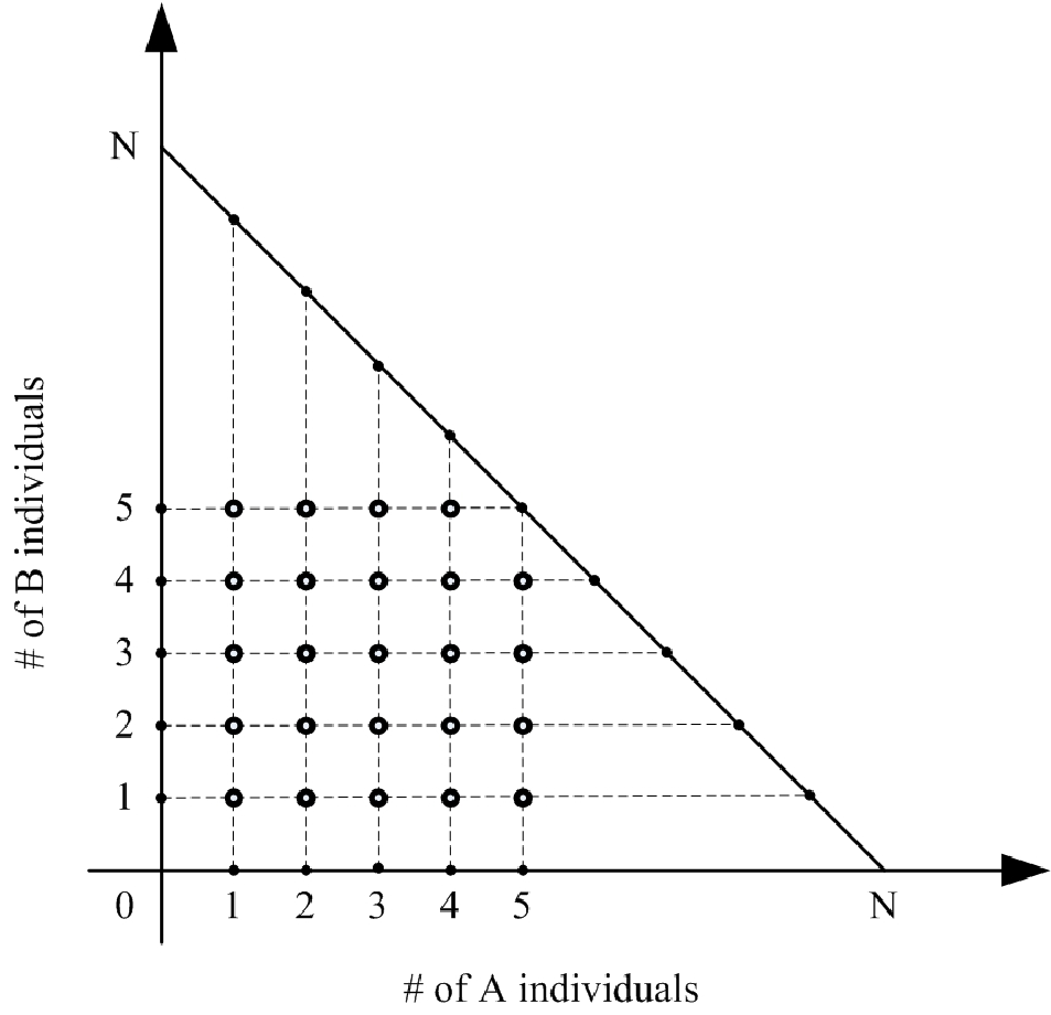
The relationship among the solutions of the system of equations can
be depicted by Fig. 1. The point marked by full black
dot denotes the boundary condition of the equations, while this
marked by empty dot denotes the unknown of the equations. Thus in
what follows, the unknown element of our interest is
discussed.
Eq. 5 can be transformed to Eq. 6 which is a system of linear equations in variables.
| (6) |
Where , . Accordingly, Eq. 5 can also be simplified to , where is a vector , is the corresponding coefficient dimensional matrix, is the corresponding vector composed of these boundary conditions. Matrix can be written as follows:
| (7) |
Here states a block of matrix
.
For fixed , in the sub-vector
, there exist a maximal
probability and a minimal probability .
They both play significant roles in the evolution process. Note that
in evolutionary dynamics, we have , . If a single individual
can be favored to replace or , more than one individuals
are more likely to replace or . Thus we only focus on the
fixation probabilities . For a neutral mutant, the fixation
probability is . When , natural selection favors
replacing or . We define as global
fixation probability and as local fixation
probability of individuals. If , natural
selection favors replacing or no matter what the ratio
of to is , that is global. Similarly, if
, the selection favors replacing or in
some proper ratios of to , not any ratios, that is local. Accordingly, there may be
three situations:
if , natural selection never favors
replacing and ;
if , natural selection always favors
replacing or whatever the ratio of to is. It is
likely that could invade the population;
if and , natural selection
favors replacing or in some proper ratios of to .
Thus the fixation of is possible under some suitable
conditions.
Let us compare the evolutionary game dynamics in infinite
populations with that in finite populations. The finite size effects
bring stochastic factor to the evolution. individuals which are
eliminated in infinite populations may be favored by natural
selection replacing or individuals. In Fig. 2, the
left column shows evolutionary game with a small frequency of
individuals initially in infinite populations, and the right column
shows that with a single individual at first in finite
populations. The first row shows situations with payoff matrix , the size .
individuals will disappear in infinite populations no matter how
many and individuals are initially. While in finite
populations, the selection won’t favor replacing or . The
second row shows the situations with payoff matrix , the size .
individuals will always invade the population of and
individuals in infinite populations. And in finite populations,
natural selection will all the time favor replacing or
no matter what the ratio of to is. The third row shows
situations with payoff matrix . individuals will disappear in infinite
populations no matter how many and individuals are
initially. Furthermore, from plenty of computations, we find that
individuals will monotonously decrease to zero in infinite
situation. Whereas sometimes will tend to replace or in finite populations.


For the three payoff matrixes in Fig. 2, it is clear that the
fixation probability of individual is not always monotonic
function of the number of individuals (see Fig. 3). Thus,
the global and local fixation probability of may
nontrivially occur
at intermediate ratio of B to C, not always end points of the ratio range of B to C.

3 AllC-AllD-TFT
Let us consider a very interesting and famous repeated game with three strategies AllC (cooperate all the time), AllD (defect all the time) and TFT (tit-for-tat). TFT is an adaptive cooperative strategy which is one of the most successful strategies proved by experiments. Individuals using TFT cooperate in the first round generally, and then do whatever the opponents did in the previous round. The number of rounds , by definition, can be . If the rounds are infinite, this game is out of our consideration. In one-round repeated Prisoners’ Dilemma game, a cooperator can obtain a benefit of or if it meets a cooperator or defector, meanwhile, it must cost whomever its opponent is; a defector can obtain a benefit of or if it meets a cooperator or defector, but costs nothing in the whole process. We bring the ratio of cost to benefit, by definition, ([0,1]), into our game, the payoff matrix between cooperator and defector can be simplified as follows:
Thus the payoff matrix of TFT, AllC and AllD with rounds is
The pairwise comparison of the three strategies leads to the
following conclusions.
(1) AllC is dominated by AllD, which means it is best to play AllD
against both AllC and AllD;
(2) TFT is equal to AllC when TFT plays with AllC;
(3) If the average number of rounds exceeds a minimum value,
, then TFT and AllD are bistable.
Suppose that a single individual using strategy TFT is brought in
the population in which some individuals adopt strategy AllC and the
others use strategy AllD originally. Provided that the number of
rounds is finite and greater than , the strategies TFT and
AllD are both strict Nash equilibrium and evolutionary stable
strategies (ESS) [2]. If , TFT becomes strategy which
is out of our discussion. Thus we need finite . For a fixed
number of individuals and a value of the rounds, we find that there
is a barrier of which can determine whether or not the selection
favors TFT replacing AllC or AllD. The barrier also has two types:
one is , which represents the barrier of local
situation; the other is , which represents that of global situation. If , the natural selection favors TFT
replacing AllC or AllD locally, whereas if , TFT
tends to be washed out by selection. The results about are
similar. Under the condition of weak selection, for sufficiently
large population size and large number of rounds , the
barrier ratio as the function of is approximately followed
by , here is a parameter dependent with
. In Fig. 4, we can fit and as
, and . In general, for
, sufficiently large and large , from abundant numeric
computations, we obtain and
, here is also a parameter
dependent with and . Thereforce, .
In other words, the ratio which could lead the selection to
favor TFT replacing AllC or AllD
globally can also induce local replacement, but not vice versa.

Deterministic replicator dynamics with three strategies in infinite
populations admits two interior equilibria at frequency of TFT given
by and . For local
situation, substitude into and , we
get and ; for global situation,
substitude into and , we
obtain and . If
the frequency of TFT at the equilibrium is or
in infinite populations, it will be favored
replacing AllC or AllD locally in finite situation; if the
frequency of TFT at the equilibrium of infinite situation is
or , it will tend
to replace AllC or AllD globally by TFT in finite
populations.
The 1/3 law proposed by Nowak in [12] is still valid in our
case, that is, the selection favors TFT replacing AllC or AllD in
finite populations, if its frequency at the equilibrium is
in infinite populations. However, when there are three
strategies TFT, AllC and AllD, in which TFT’s frequency at one
equilibrium is , the corresponding frequency of AllC is zero.
Thus in this situation, our results to some extent validate the
conjecture in which AllC is eliminated by natural selection so
quickly that the effect of AllC can be neglected in finite
populations. And then the evolutionary game dynamics with the two
left strategies TFT and AllD, is equivalent to the situation of the
situation with these two strategies initially. Nevertheless not any
size of AllC individuals could be wiped out quickly, their effects
can not be ignored in the dynamics. Hence can only
determine the replacement locally (in some certain
circumstances). As for global fixation situation (the fixation
is certain for any ratio of AllC to AllD), we have
for . The conditions that
natural selection favors global replacement of AllC or AllD by
TFT are more intensified than
those of local situation.
Let us discuss the other equilibrium. The is a
monotony increasing function of . This approaches
one for increasing . That is to say, when the number of rounds
increases, the condition can be satisfied with
higher probability, and TFT may have more opportunities to replace
AllC or AllD locally and globally. In the standard
evolutionary model of the finitely repeated Prisoner’s Dilemma, TFT
can not invade AllD. But interestingly, we find that for
intermediate , if , nature selection favors
TFT replacing AllC or AllD as the fixation probability of a single
TFT () is larger than that of a single AllC
() or AllD (). Actually, in this case,
. Therefore, a single
TFT is likely to invade the entire population consisting of AllC and
AllD finally. In this case, cooperation tends to emerge in the
evolution process. And yet, for large limit , the situation is
out of our consideration due to its extraordinary intricacy.
However, as increasing to infinite, the probability that the
selection favors TFT taking over the whole population also
approaches one. Accordingly, the fixation of cooperation is enhanced
in finite populations. It is because that when TFT meets AllD, its
loss in the first round can be diluted by many rounds games. In this
case, the total fitness of TFT is almost the same as that of AllD
and they are a pair of nip and tuck opponents. But TFT receives more
payoff than AllD when they both play with TFT. To sum up, TFT is
superior to AllD for limit large rounds because of its adaption. As
a result of this property of TFT, natural selection mostly prefers
to choose TFT to reproduce offspring, and then TFT is most likely to
dominate the population at last. Therefore, cooperation has more
opportunities to win in finite populations contrasting against
infinite situation.
4 Conclusion
We have proposed a model of evolutionary game dynamics with three
strategies in finite populations. It can be characterized by a
frequency-dependent Moran process which could be stated by a system
of linear equations. By the comparative study of evolution in finite
and infinite populations, we shew that a single individual which
can not invade infinite populations may have an opportunity to
replace or in finite situation. In other words, a single
individual could be eliminated by selection with smaller probability
in finite populations than situation in infinite populations. In
addition, a famous game with AllC, AllD, and TFT is adopted to
illuminate our results by numeric computations. Furthermore, under
the condition of weak selection, for sufficiently large population
size and appropriate number of rounds , a single TFT could
invade the population composed of AllC and AllD with high
probability almost one. In this situation, the emergence of
cooperation is attributed to the finite population size effects. Our
results may help understand the
coevolution of multi-species and diversity of natural world.
Acknowledgement
We are grateful to Xiaojie Chen and Bin Wu for helpful discussions and comments. This work was supported by National Natural Science Foundation of China (NSFC) under grant Nos. 60674050 and 60528007, National 973 Program (Grant No.2002CB312200), National 863 Program (Grant No.2006AA04Z258) and 11-5 project (Grant No. A2120061303).
References
- [1] R. C. Lewontin, J. Theor. Biol. 1 (1961) 382.
- [2] J. Maynard Smith, Evolution and the Theory of Games, Cambridge University Press, Cambridge, UK, 1974.
- [3] J. Hofbauer and K. Sigmund, Evolutionary Games and Population Dynamics, Cambridge University Press, Cambridge, UK, 1998.
- [4] R. Cressman, Evolutionary Dynamics and Extensive Form Games, MIT Press, Cambridge, MA, 2003.
- [5] P. D. Taylor and L. Jonker, Math. Biosci. 40 (1978) 145.
- [6] D. Neal, Introduction to Population Biology, Cambridge University Press, Cambridge, UK, 2004.
- [7] M. Benaim and J. Weibull, Econometrica 71 (2003) 873.
- [8] A. Traulsen, J. C. Claussen and C. Hauert, Phys. Rev. Lett. 95 (2005) 238701.
- [9] J. C. Claussen and A. Traulsen, Phys. Rev. E. 71 (2005) 025101(R).
- [10] N. G. van Kampen, Sochastic Processes in Physics and Chemistry, 2nd ed, Elsevier, Amsterdam, 1997.
- [11] A. Traulsen, J. C. Claussen and C. Hauert, Phys. Rev. E 74 (2006) 011901.
- [12] M. A. Nowak, A. Sasaki, C. Taylor and D. Fudenberg, Nature (London) 428 (2004) 646.
- [13] C. Taylor, D. Fudenberg, A. Sasaki and M. A. Nowak, Bull. Math. Biol. 66 (2004) 1621.
- [14] D. Fudenberg, M. A. Nowak, C. Taylor and L. Imhof, Theor. Pop. Biol. 70 (2006) 352.
- [15] P. A. P. Moran, The Statistical Processes of Evolutionary Theory, Clarendon Press, Oxford, 1962.
- [16] S. Karlin, H. M. Taylor, A First Course in Stochastic Processes, 2nd ed, Academic Press, New York, 1975.
- [17] L. A. Imhof, D. Fudenberg and M. A. Nowak, Proc. Natl. Acda. Sci. USA 102 (2005) 10797.
- [18] E. Lieberman, C. Hauert and M. A. Nowak, Nature (London) 433 (2005) 312.
- [19] C. Taylor, Y. Iwasa and M. A. Nowak, J. Theor. Biol. 243 (2006) 245.
- [20] T. Antal and I. Scheuring, Bull. Math. Biol. 68 (2006) 1923.
- [21] L. A. Imhof and M. A. Nowak, J. Math. Biol. 52 (2006) 667.
- [22] A. Traulsen, M. A. Nowak and J. M. Pacheco, Phys. Rev. E 74 (2006) 011909.
- [23] T. Antal, S. Redner and V. Sood, Phys. Rev. Lett 96 (2006) 188104.
- [24] H. Ohtsuki, C. Hauert, E. Lieberman and M. A. Nowak, Nature (London) 441 (2006) 502.
- [25] B. Kerr, M. A. Riley, M. W. Feldman and B. J. M. Bohannan, Nature (London) 418 (2002) 171.