Mean Flow of Turbulent-Laminar Patterns
in Plane Couette Flow
Abstract
A turbulent-laminar banded pattern in plane Couette flow is studied numerically. This pattern is statistically steady, is oriented obliquely to the streamwise direction, and has a very large wavelength relative to the gap. The mean flow, averaged in time and in the homogeneous direction, is analysed. The flow in the quasi-laminar region is not the linear Couette profile, but results from a non-trivial balance between advection and diffusion. This force balance yields a first approximation to the relationship between the Reynolds number, angle, and wavelength of the pattern. Remarkably, the variation of the mean flow along the pattern wavevector is found to be almost exactly harmonic: the flow can be represented via only three cross-channel profiles as . A model is formulated which relates the cross-channel profiles of the mean flow and of the Reynolds stress. Regimes computed for a full range of angle and Reynolds number in a tilted rectangular periodic computational domain are presented. Observations of regular turbulent-laminar patterns in other shear flows – Taylor-Couette, rotor-stator, and plane Poiseuille – are compared.
www.maths.warwick.ac.uk/barkley
barkley@maths.warwick.ac.uk
2 LIMSI-CNRS, BP 133, 91403 Orsay, France
www.limsi.fr/Individu/laurette
laurette@limsi.fr
1 Introduction
Pattern formation is associated with the spontaneous breaking of spatial symmetry. Many of the most famous and well-studied examples of pattern formation come from fluid dynamics. Among these are the convection rolls which spontaneously form in a uniform layer of fluid heated from below and the Taylor cells which form between concentric rotating cylinders. In these cases continuous translational symmetries are broken by the cellular flows beyond critical values of the control parameter – the Rayleigh number or Taylor number.
A fundamentally new type of pattern has been discovered in large-aspect-ratio shear flows in recent years by researchers at GIT-Saclay Prigent & Dauchot 2000; Prigent et al. 2002; Prigent et al. 2003; Prigent & Dauchot 2005; Bottin et al. 1998. Figure 1 shows an example from plane Couette experiments performed by these researchers. One sees a remarkable spatially-periodic pattern composed of distinct regions of turbulent and laminar flow. The pattern itself is essentially stationary. The pattern wavelength is large compared with the gap between the plates and its wavevector is oriented obliquely to the streamwise direction.
The pattern emerges spontaneously from featureless turbulence as the Reynolds number is decreased. This is illustrated in figure 2 with time series from our numerical simulations of plane Couette flow for decreasing Reynolds number (conventionally defined based on half the velocity difference between the plates and half the gap). At Reynolds number 500, the flow is uniformly turbulent. Following a decrease in the Reynolds number below 400 (specifically 350 in figure 2) the flow organises into three regions of relatively laminar flow and three regions of more strongly turbulent flow. While the fluid in the turbulent regions is very dynamic, the pattern is essentially steady.
Shear flows exhibiting regular coexisting turbulent and laminar regions have a been known for many years. In the mid 1960’s, a state known as spiral turbulence was discovered Coles 1965; van Atta 1966; Coles & van Atta 1966 in counter-rotating Taylor-Couette flow. Consisting of a turbulent and a laminar region, each with a spiral shape, spiral turbulence was further studied in the 1980s Andereck et al. 1986; Hegseth et al. 1989. Experiments by the Saclay researchers Prigent & Dauchot 2000; Prigent et al. 2002; Prigent et al. 2003; Prigent & Dauchot 2005 in a very large aspect-ratio Taylor-Couette system have shown that the turbulent and laminar regions in fact form a periodic pattern, of which the original observations of Coles and van Atta comprised only one wavelength. Analogues of these states occur in other shear flows as well. Cros & Le Gal 2002 discovered large-scale turbulent spirals in the shear flow between a stationary and a rotating disk. Tsukahara et al. 2005 observed oblique turbulent-laminar bands in plane Poiseuille flow. A unified Reynolds number based on the shear and the half-gap can be defined for these different flows Prigent et al. 2003 and is described in the Appendix. When converted to comparable quantities in this way, the Reynolds-number thresholds, wavelengths, and angles are similar for all of these turbulent patterned flows. The patterns are always found near the minimum Reynolds numbers for which turbulence can exist in the flow.
In this paper we present a detailed analysis of these turbulent-laminar patterns. We will focus on a single case – the periodic pattern at Reynolds number 350. From computer simulations, we obtain the flow and identify the symmetries of the patterned state. We consider in detail the force balance responsible for maintaining the pattern. From the symmetries and harmonic content we are able to reduce the description to six ordinary-differential equations which very accurately describe the patterned mean flow.


2 Preliminaries
2.1 Geometry
The unusual but key feature of our study of turbulent-laminar patterns is the use of simulation domains aligned with the pattern wavevector and thus tilted relative to the streamwise-spanwise directions of the flow. Figure 3 illustrates this and defines our coordinate system. In figure 3(a) a simulation domain is shown as it would appear relative to an experiment, figure 1, in which the streamwise direction (defined by the direction of plate motion) is horizontal. The near (upper) plate moves to the right and the far (lower) plate to the left in the figure. As we have discussed in detail Barkley & Tuckerman 2005a; Barkley & Tuckerman 2005b, simulating the flow in a tilted geometry has advantages in reducing computational expense and in facilitating the study of pattern orientation and wavelength selection. The important point for the present study is that the coordinates are aligned to the patterns. The direction is parallel to the pattern wavevector while the direction is perpendicular to the wavevector (compare figure 3(a) with figure 1).
Figures 3(b) and (c) show the simulation domain as it will be oriented in this paper. In this orientation the streamwise direction is tilted at angle (here ) to the direction. This choice of angle is guided by the experimental results and by our previous simulations. (In past publications Barkley & Tuckerman 2005a; Barkley & Tuckerman 2005b we have used un-primed coordinates for those aligned along spanwise-streamwise directions and primes for coordinates tilted with the simulation domain. Here we focus exclusively on coordinates fixed to the simulation domain and so for convenience denote them without primes.) In these tilted coordinates, the streamwise direction is
| (1) |
where
| (2) |
We take , for the reasons explained in Jiménez & Moin 1991; Hamilton et al. 1995; Waleffe 2003; Barkley & Tuckerman 2005a; Barkley & Tuckerman 2005b. Essentially, must be near 4 in order to contain one pair of streaks or spanwise vortices, which are necessary to the maintenance of low Reynolds number wall-bounded turbulence. Although our simulations are in a three-dimensional domain, we will average the results in the homogeneous direction, as will be explained in section 2.3. For most purposes it is sufficient to view the flow in the coordinates illustrated in figure 3(c). The midplane between the plates corresponds to .
The length of our computational domain is guided by the experimental results and by our previous simulations. One of the distinctive features of the turbulent-laminar patterns is their long wavelength relative to the gap between the plates. A standard choice for length units in plane Couette flow is the half-gap between the plates. In the simulation with and shown in figure 2, a pattern of wavelength 40 emerged spontaneously from uniform turbulence when the Reynolds number was lowered to . For this reason, the simulations we will describe below are conducted with . The corresponding wavenumber is
| (3) |
This large wavelength, or small wavenumber, expresses the fact that the pattern wavelength in is far greater than the cross-channel dimension.

2.2 Equations and Numerics
The flow is governed by the incompressible Navier–Stokes equations
{subeqnarray}
u
t
= -(u⋅∇)u- ∇p +
1
Re
∇^2u in ,
0=∇⋅u in ,
where is the velocity field and is the static
pressure. Without loss of generality the density is taken to be one. The
equations have been nondimensionalized by the plate speed and the half gap
between the plates. is the tilted computational domain discussed
in the previous section.
No-slip boundary conditions are imposed at the plates and periodic boundary
conditions are imposed in the lateral directions. In our coordinates the
conditions are
{subeqnarray}
u(x,y=±1,z) = ±(e_xcosθ+ e_zsinθ)
u(x + L_x,y,z) = u(x,y,z)
u(x,y,z + L_z) = u(x,y,z).
Linear Couette flow is a solution to (2.2)–(2.2), which is stable for all Re and satisfies
| (4) |
In our tilted coordinate system,
| (5) |
The Navier-Stokes equations (2.2) with boundary conditions (2.2) are simulated using the spectral-element (-) – Fourier () code Prism Henderson & Karniadakis 1995. We use a spatial resolution consistent with previous studies Hamilton et al. 1995; Waleffe 2003. Specifically, for a domain with dimensions and , we use a computational grid with 10 elements in the direction and 5 elements in the direction. Within each element, we use th order polynomial expansions for the primitive variables. In the direction, a Fourier representation is used and the code is parallelized over the Fourier modes. Our domain with is discretized with 512 Fourier modes or gridpoints. Thus the total spatial resolution we use for the domain can be expressed as modes or gridpoints.
2.3 Dataset and averaging
The focus of this paper is the mean field calculated from the simulation illustrated by the spatio-temporal diagram in figure 5(a). The velocity field in the portion of the domain shows high-frequency and high-amplitude fluctuations, while the flow in the right portion is basically quiescent. We will call the flow on the left turbulent, even though it could be argued that it is not fully developped turbulence. We will call the flow on the right laminar, even though occasional small fluctuations can be seen in this region.
The turbulent-laminar pattern subsists during the entire simulation of time units. However the pattern undergoes short-scale “jiggling”, seen particularly at the edges of the turbulent regions, and longer-scale drifting or wandering in the periodic direction. We seek to describe the field which results from smoothing the turbulent fluctuations, but for which drifting is minimal, by averaging over an appropriate time interval. The desired averaging time interval represents a compromise between the short and long timescales. We have chosen to average the flow in figure 5(a) over the shaded time interval , during which the pattern is approximately stationary.
The time-averaged flow is homogeneous in -direction. This is illustrated in figure 5(b) where we plot one of the velocity components time-averaged flow over the interval . Cuts at different locations show that there is essentially no variation in the -direction. All other quantities are similarly independent of . It is therefore appropriate to consider mean flows as averages over the direction as well as over the time.
We define mean flows as
{subeqnarray}
⟨u⟩(y,z) ≡
1
T
1
L
x
∫_t^t+T
∫_0^L_x u(x,y,z,t) dx dt
⟨p ⟩(y,z) ≡
1
T
1
L
x
∫_t^t+T
∫_0^L_x p(x,y,z,t) dx dt.
The mean fields obey the averaged Navier-Stokes equations
{subeqnarray}
0=-(⟨u⟩⋅∇) ⟨u⟩- ⟨(
~
u
⋅∇)
~
u
⟩-∇⟨p ⟩+
1
Re
∇^2⟨u⟩
0=∇⋅⟨u⟩,
where
| (6) |
is the fluctuating field and denotes - average. The mean fields are subject to the same boundary conditions as equations (2.2). We denote the Reynolds-stress force from the fluctuating field in equations (2.3) by :
| (7) |
We shall focus almost exclusively on the difference between the mean flow and linear Couette flow, for which we introduce the notation
| (8) |
as well as .
Letting the components of be denoted by and the components of be denoted by , then the averaged Navier-Stokes equations for the deviation from linear Couette flow in component form become
| (9a) | |||||
| (9b) | |||||
| (9c) | |||||
| (9d) | |||||
is required to satisfy homogeneous boundary conditions at the plates
| (10) |
and periodic boundary conditions in .
A system of this type, with three components depending on two coordinates, is sometimes called 2.5 dimensional. The transverse, or out-of-plane flow appears only in the first equation and is effectively a passive scalar advected by the in-plane flow and driven by the Reynolds-stress force . The in-plane flow can be expressed in terms of a streamfunction where
| (11) |
We shall use both and to describe the mean flows.


3 Results
We present a characterisation of the turbulent-laminar pattern at . We describe in detail the mean flow, its symmetries, and the dominant force balances within the flow. Our goal here is not to consider closures for averaged Navier-Stokes equations (9). We will make no attempt to model the turbulence, i.e. to relate the Reynolds-stress tensor to the mean flow . Instead we use fully resolved (three-dimensional, time-dependent) numerical simulations of the turbulent flow to measure both the mean field and Reynolds-stress force . From these we extract the structure of these fields and the dominant force balances at play in sustaining turbulent-laminar patterns.
3.1 Mean flow
The mean flow is visualised in figure 5 via the transverse, out-of-plane flow and the in-plane streamfunction . Recall [equation (8)] that these fields are the deviations of the mean flow from linear Couette flow . The mean turbulent kinetic energy
| (12) |
serves to clearly identify the turbulent region. In these and subsequent plots, the middle of the laminar region is positioned at the centre of the figure and the turbulent region at the periodic boundaries of the computational domain. In figure 5 (but not in subsequent figures), plots are extended in the -direction one quarter-period beyond each periodic boundary to help visualise the flow in the turbulent region. The pattern wavelength is , so that and describe the same point, as do and .
The mean flow can be described as follows. is strongest in the turbulent-laminar transition regions. In the transition region to the left of centre () in figure 5, is negative and primarily in the upper half of the channel. To the right of centre (), is positive and is seen primarily in the lower half of the channel. Comparison with turbulent kinetic energy shows that the transverse mean flow is out of phase with respect to the fluctuating field by . This has been seen experimentally by Coles & van Atta 1966 and Prigent et al. (Prigent et al. 2002, Prigent et al. 2003, Prigent & Dauchot 2005).
The in-plane flow in figure 5 has a large-aspect ratio cellular structure consisting of alternating elliptical and hyperbolic points. The flow around the elliptical points, located in the centre of the turbulent regions, rotates in a counter-clockwise sense, opposing linear Couette flow. In the vicinity of the hyperbolic points, centred in the laminar regions, the in-plane deviation from linear Couette flow is very weak ( and nearly zero).
Figure 7 shows -profiles at four key points equally spaced along the pattern: centre of the laminar region, turbulent-laminar transition region, centre of the turbulent region, and the other turbulent-laminar transition region. While the profile is plotted, its variation is very small on the scale of and and can essentially be used to indicate the axis. Figure 7 shows profiles for the full mean flow containing the linear Couette profile.


The profiles in figure 7 are S-shaped, of the type found in turbulent Couette flow. This is to be expected in the turbulent region, even at these low Reynolds numbers. However, it is very surprising that the profile in the laminar region is also of this form. In the laminar region, local Reynolds stresses are absent (see figure 5) and so cannot be responsible for maintaining the S-shaped velocity profile in the laminar regions. The other prominent features in figures 7 and 7 are the asymmetric profiles at the transition regions.
The relationship between the mean flow field and the regions of turbulence can be seen in figure 8. Here the flow is shown in the standard orientations. In each view, greyscale indicates the size of the turbulent energy and the arrows show the mean flow within the plane. In the top two views, the flow is shown in the streamwise-spanwise planes located at and at . The next view shows the flow between the plates, i.e.in a streamwise-cross-channel plane, and the last shows an enlargement of one of the laminar-turbulent transition regions. Note that the length of our tilted computational domain corresponds to a streamwise length of and to a spanwise length of .
The flow in figure 8 can be compared with the mean flow reported by Coles & van Atta 1966 in experiments on turbulent spirals in Taylor-Coutte flow. Coles and van Atta measured the mean flow near the midgap between the rotating cylinders and noted an asymmetry between the mean flow into and out of turbulent regions. They found that the mean flow into turbulent regions was almost perpendicular to the turbulent-laminar interface whereas flow out of the turbulent region was almost parallel to the turbulent-laminar interface. We also observe a striking asymmetry between the mean flow into and out of the turbulent regions. The orientation of our mean flow does not agree in detail with that of Coles and van Atta, but this is most likely due to the fact that Coles and van Atta considered circular Taylor-Couette flow and measured the flow near the mid-gap. Referring to figures 5 and 7 one sees that the mid-plane () is not the ideal plane on which to obverve the mean flow since its structure is most pronounced between the midplane and the upper or lower walls.
Before considering the symmetries and force balances in detail, it is instructive to consider the dominant force balance just at the centre of the laminar region. Recall that one of the more interesting features of the mean flow is that the profile appears very similar to a turbulent profile, even in the absence of turbulence in the laminar region. Here the balance is dominated by advection and viscous diffusion, as shown in figure 9. Equation (9a) for flow in the -direction is
| (13) |
Variations in dominate variations in , i.e. the usual boundary-layer approximation holds; see, e.g. Pope 2000. Indeed, approximating the dependence of by the functional form suggested by figure 7, we have
| (14) |
This is confirmed by the second panel of figure 9. In the centre of the laminar region , , and are all negligible, so that dominates the advective terms, as shown in the third panel of figure 9. Thus the balance between advection and viscosity in the laminar region is
| (15) |
This equation is appealingly simple and yet leads immediately to some interesting conclusions. The first is that a non-zero tilt angle is necessary to maintain the S-shaped profile in the laminar region, since otherwise and could be at most linear in and would in fact be zero, due to the homogeneous boundary conditions (10). The second conclusion follows from consideration of parity. The multiplication by on the left-hand-side reverses -parity, while the second derivative operator on the right-hand-side preserves parity. The conclusion is that should be decomposed into odd and even components in and equation (15) should actually be understood as two equations coupling the two components. Specifically, as can be seen in figure 7, is odd in in the centre of the laminar region, yet must be even for equation (15) to hold.
The remainder of the paper is devoted to formalising, demonstrating and extending this basic idea.

3.2 Symmetry and Fourier modes
We now consider in depth the symmetry properties of the flow. We start with the symmetries of the system before averaging, that is, the Navier-Stokes equations (2.2) and boundary conditions (2.2). The system has translation symmetry in and as well as centrosymmetry under combined reflection in , and :
| (16) |
where the origin , can be chosen arbitrarily. Linear Couette flow possesses all the system symmetries, as does the mean flow at Reynolds numbers for which turbulence is statistically homogeneous in and .
Note that in the absence of tilt (), the system possesses two reflection symmetries. These can be taken to be and reflection in the spanwise direction. For the tilted domain (at angles other than multiples of ), the only reflection symmetry is . This can be seen in figure 3(a): for general tilt angles , spanwise reflection does not preserve the domain, i.e. does not leave the periodic boundaries in place. The experimental system shown in figure 1 possesses spanwise reflection symmetry and hence bands can be observed in the either of the two symmetrically related angles, the choice is dictated by factor such as initial conditions. By design, our tiled computational domain precludes the symmetry-related pattern given by spanwise reflection.
The transition to the turbulent-laminar patterned state breaks symmetry. Specifically, both the mean flow and the Reynolds-stress force break -translation symmetry but break neither -translation symmetry nor centrosymmetry. The spatial phase of the pattern in is arbitrary, but given a phase there are two values of , separated by half a period, for which the flow is invariant under , as is typical for a circle pitchfork bifurcation Crawford & Knobloch 1991. As can be seen in figure 5, the values of about which the patterns are centrosymmetric are the centres of the laminar () and of the turbulent () regions.
The centrosymmetry operator for our averaged fields , which depend only on and , is
| (17) |
Since the Reynolds-stress force is centrosymmetric in the case we consider, then the averaged equations (9) for the mean field have centrosymmetry.
We formalise this further as follows. Any -independent field can be decomposed into even and odd functions of and as
| (18) |
where, for example, is odd in and even in . Applying the operator in (17) to (18), we obtain
| (19) | |||||
For the field to be centrosymmetric requires , so that in fact
| (20) |
Table 1, as well as figure 5, shows that this is indeed the case for ; it holds for as well.
We now Fourier transform in to further decompose the mean velocity and the Reynolds-stress force. We find that the -wavenumbers and have contributions to which are an order of magnitude higher than the remaining wavenumber combinations. See table 2. The deviation from the average is thus almost exactly trigonometric, with almost no higher harmonic content. The dominance of these terms in the Fourier series means that and can be represented by only three functions of , namely:
| (30) |
which is a special case of (20), with the first two terms of (30) coinciding with and the last to . Thus, and are odd functions of , while is even. The fields thus consist of a -independent component and two components which vary trigonometrically and out of phase with one another, dominating in the laminar and turbulent regions and dominating in the boundaries between them. Moreover, dominates in the bulk, since and are odd in and thus zero in the channel centre.
| Centre of laminar region | (31a) | ||||||
| Laminar-turbulent boundary | (31b) | ||||||
| Centre of turbulent region | (31c) | ||||||
| Turbulent-laminar boundary | (31d) | ||||||
Figure 10 shows the three trigonometric components, each a function of , obtained by Fourier transforming , , and . Figure 11 shows , and as functions of at locations in the upper and lower channel and compares them with the values obtained from the trigonometric formula (30) using the functions shown in figure 10. Figures 14, 14 and 14 depict , and with their trigonometric decompositions. Each of these figures uses only the three scalar functions of , figure 10, to reproduce the corresponding two-dimensional field. As shown by equation (11), the streamfunction of a centrosymmetric field has symmetry opposite to that of the velocity components, i.e. it is composed of functions of the same parity in and .


Figures 15 and 16 show the three Reynolds-stress forces and their Fourier decompositions. Each component obeys , a necessary condition for to vanish at the centre of the laminar region, as shown by equation (31a) and also illustrated in figure 14. More precisely,
| (32) |
In addition,
| (33) |
as is typical for turbulent channel flows; see, e.g. Pope 2000.


3.3 Force balance for
We now turn to understanding the balance of forces responsible for maintaining the mean flow profiles. We focus primarily on , both because it is the component of largest amplitude and also because it appears only in equation (9a): is subject to Reynolds-stress and viscous forces, and is advected by but is not self-advected. We begin by showing the balance of forces in the direction as a function of at locations in the upper and lower channel in figure 17. One can again see the centrosymmetry of each of the forces, i.e. invariance under the combined operations of reflection in and and change of sign. The Reynolds-stress force disappears at the center of the laminar region and the advective and viscous forces exactly counterbalance, as emphasized in the figures on the right. Figure 20 shows another view of this balance, displaying the forces as a function of at four locations in . As previously stated, is dominated by and by . In figure 20, we show the Fourier-space analogue of figure 20.


We now turn to the more complex advective forces, whose Fourier decompositions are shown in figure 20. The component of the advective force is small but non-zero. Because this term results from the product of trigonometric functions, it also provides a measure of the generation of higher harmonics, a point which we will explore further in section 3.5. The advective term is well approximated by the contribution from advection by . The advective term is dominated near the walls by advection by , but in the bulk by advection by . Properties of the and modes echo their physical space counterparts: the advective term is well approximated by advection by in the laminar region, as was shown in figure 9, while the advective forces in the laminar-turbulent boundaries combine advection by near the walls and by in the bulk.
We illustrate these conclusions via schematic visualizations of the dynamics of . Figure 21 illustrates the dynamics in the laminar and turbulent regions. The dynamics in the laminar region are essentially described by the simple balance between viscous diffusion of profiles and advection by linear Couette flow in , given by equation (15). Viscous diffusion tends to reduce curvature, but the profiles have greater curvature upstream (to the left for the upper channel, to the right for the lower channel). Hence advection replenishes the curvature damped by viscosity. However, this trend towards greater curvature upstream cannot continue indefinitely, since the pattern is periodic in . Hence eventually a maximum is reached (at a turbulent-laminar boundary), beyond which the curvature decreases upstream. Thus, in the turbulent region, advection and diffusion act together to decrease curvature and must both be counter-balanced by turbulent forcing. These features are essentially described by the and modes. Figure 22 illustrates the dynamics in the turbulent-laminar boundaries. These dynamics include advection by in the bulk, leading to the () patch in the lower right (upper left) of figure 14 and are described by the mode.


3.4 Force balance for and


Figure 25 shows the balance of forces in the direction and figure 25 its analogue in Fourier space. This balance resembles that in the direction shown in figures 20 and 20. In physical space (compare the leftmost panels of figures 25 and 20), the main difference is that the advective and viscous forces are both small in the laminar region, in keeping with the fact that . The pressure gradient is far smaller than the other forces throughout (see below). In Fourier space (compare the middle panels of figures 25 and 20), the main difference with the balance is that the relative importance of the viscous and advective forces in the balance is reversed from that in the case of : for , the viscous component is larger than the advective component, which is especially small in the bulk. The decomposition of the advective terms (figure 25) shows that, as is the case for , the advective term is well approximated by the contribution from advection by , whereas all four advective components contribute to the term.
The balance of forces in the direction is entirely different. The dominant balance in this equation is:
| (34) |
as shown in figure 26. This is typical for turbulent channel flows; see, e.g. Pope 2000. This balance between the mean pressure gradient and the Reynolds-stress force does not constrain or provide information about any of the velocity components. Since
| (35) |
we in fact have
| (36) |
up to a small -dependent correction. Figure 5 shows the pressure field calculated from (36) and suggests that its dependence can be approximated by the functional form . This leads to an estimate of the relative importance of the pressure gradients in the and directions:
| (37) |
while our data shows
| (38) |
The same estimate applies to the relative magnitudes of and , using the streamfunction shown in figure 5:
| (39) |
while the actual ratio of maximum values is
| (40) |

3.5 Model equations
We now derive a system of ordinary differential equations by substituting the trigonometric form (30) into the Reynolds-averaged Navier-Stokes equations (9). The drawback in this procedure is the usual one, namely that this form is not preserved by multiplication. However, Table 2 shows that higher harmonics contribute very little to .
We expand the advective term as:
| (41a) | |||||
| (41b) | |||||
| (41c) | |||||
| (41d) | |||||
where primes denote differentiation. We neglect the second harmonic term (41d), and will discuss the accuracy of this approximation below. We now rewrite the and components of the averaged momentum equations, neglecting the -derivatives , and , as justified by equations (14) and (37):
| (42a) | |||||
| (42b) | |||||
Substituting (41a)–(41c) in (42) and separating terms in , and , we obtain
| (43a) | |||||
| (43b) | |||||
| (43c) | |||||
| (43d) | |||||
| (43e) | |||||
| (43f) | |||||
where the Fourier modes of and are related via those of the streamfunction of (11):
| (44a) | |||||
| (44b) | |||||
| (44c) | |||||
and where homogeneous boundary conditions are imposed:
{subeqnarray}
0= U_0 = U_c = U_s at y=±1
0= W_0 = W_c = W_s at y=±1
System (43) with boundary conditions (3.5) is composed of six ordinary differential equations coupling the six scalar functions of , with six turbulent forces .
We have solved (43)–(3.5) numerically, using as inputs and obtained from our full simulations, i.e. the modes shown in figure 16. The resulting solutions are shown in figure 27. For comparison, we reproduce from figure 10 the mean velocity fields, in Fourier representation, from our full simulations (DNS). The ODE solutions are virtually indistinguishable from the mean fields from DNS. Only in the sine component of can the ODE solutions be distiguished (and only very slightly) from the DNS results. From the profiles in figure 27, the full mean fields could be constructed as in figures 14 and 14. Thus, while the ODE model requires input of the Reynolds-stress force terms, and , it demonstrates the simplicity of the force balance responsible for generating the patterned flow when viewed in the Fourier representation. Considering higher harmonics would be straightforward, but would serve little purpose.

We can go in the other direction and attempt to simplify system (43). The approximate equalities , [see equation (32)], necessary for to vanish at the center of the laminar region, can be imposed exactly, reducing the number of turbulent forcing input functions to four. The terms arising from the advective forces can be reduced by making approximations justified from figures 20 and 25. The nonlinear terms in (43a) and (43d) can be neglected. The advective terms in (43b) and (43e) can be approximated by and . Making these approximations, we obtain:
| (45a) | |||||
| (45b) | |||||
| (45c) | |||||
| (45d) | |||||
| (45e) | |||||
| (45f) | |||||
The solutions to this simplified ODE model are also presented in figure 27. There is quite good agreement with full DNS results, thus demonstrating that the dominant force balance is captured by this very simple system of ODEs. We stress that the only nonlinearities in this model are in equations (45c) and (45f). This reflects the complexity of the dynamics in the turbulent-laminar boundaries regions (and the simplicity of the dynamics in the centre of the turbulent and laminar regions.)
4 Discussion
We have presented an analysis of a particular turbulent-laminar pattern obtained in simulations of large-aspect-ratio plane Couette flow. We have focused on a single example so as to understand in quantitative detail the structure of these unusual flows. The key findings obtained in our study are as follows. First we find that in the (quasi-) laminar flow region the velocity profiles are not simply those of linear Couette flow. Instead a non-trivial flow is maintained in the laminar regions by a balance between viscous diffusion and nonlinear advection. Next we have considered the symmetries of the flow. When the pattern forms, the time-averaged flow breaks the translation symmetry but not centrosymmetry. The patterned state is centrosymmetric about the centre of the laminar region and about the center of the turbulent region. Next we have considered a spatial Fourier decomposition of the mean flow in the direction of the pattern wavevector. From this we find that the lateral structure of the pattern is almost completely harmonic, i.e. composed of a constant and single harmonic. Thus the pattern description can be reduced to just three cross-channel functions for each field, in that . The absence of higher harmonics suggests that the pattern is near the threshold, in some sense, of a linear instability of a uniform turbulent state. Such an instability would be governed by a linear equation with coefficients which are constant in , whose solutions are necessarily trigonometric in .
From our analysis of the turbulent-laminar pattern, in particular its Fourier decomposition, we derive a model which reproduces the patterned flow. The model is derived from the averaged Navier-Stokes equations with the following assumptions. The crucial assumption, which is strongly supported by our numerical computations, is that the mean flow can be expressed in terms of just three horizontal modes. Effectively the generation of higher harmonics via nonlinear terms in the Navier-Stokes equations is negligible in the mean flow. The model is then further simplified because viscous diffusion is dominated by cross-channel diffusion – the standard boundary-layer approximation – and because pressure variation is negligible along the pattern wavevector. We take as input to the model the Reynolds-stress forces measured from computations. Assuming that the Reynolds stresses exactly vanish in the centre of the laminar regions, the number of inputs to the model is just four cross-channel functions. The result is a system of six simple ordinary differential equations which depend on four forcing functions. The model equations accurately reproduce the mean flow from full direct numerical simulations.
A number of other researchers have attempted to reduce the description of turbulent or transitional plane Couette flow by various means. At these low Reynolds numbers, there is no doubt that fully resolved direct numerical simulation is feasible and gives accurate results. The purpose of formulating a reduced description is therefore to yield understanding. We now comment on the differences between the approaches used by other authors and our reduction.
In parallel with their experiments, Prigent et al. (Prigent et al. 2002; Prigent et al. 2003) considered a pair of coupled Ginzburg-Landau (GL) equations with additive noise as a model for the transition from uniform turbulence to turbulent-laminar banded patterns via noisy (intermittent) patterns. These equations describe the variation in time and spanwise coordinate of the amplitudes of two sets of laminar bands at opposite tilt angles. These laminar bands modulate the uniform turbulence in competition with one another. Each equation separately has one reflection symmetry which corresponds physically to the centrosymmetry (equation (17)) of a banded pattern. The coupled GL equations possess a second reflection symmetry, corresponding physically to a spanwise reflection, which takes the amplitude to and vice versa. By design, this symmetry is not present in our numerical computations. Prigent et al. used their experimental results to fit the parameters in the GL equation and then compared simulations of the equations with experimental results. Steady patterns in the resulting GL equations have only one non-zero amplitude and this amplitude possesses the reflection symmetry corresponding to . Hence, the steady patterns in these simulations have exactly the symmetries of the patterns we have considered.
An important class of models aims at reproducing dynamics of streamwise vortices and streaks in plane Couette turbulence by using a small number of ordinary differential equations (ODEs). These equations describe the time-evolution of amplitudes of modes with fixed spatial dependence. Waleffe 1997, guided by the discovery of the self-sustaining process (SSP) in direct numerical simulations Hamilton et al. 1995, derived a system of eight ODEs, whose variables represent amplitudes of the key ingredients of the SSP, namely longitudinal vortices, streaks, and streak waviness. This model was later also studied and extended by Dauchot & Vioujard 2000 and by Moehlis et al. 2004.
Two other Galerkin projection procedures have been used to derive ODE models. The most energetic streamwise-independent modes in a principle orthogonal composition has been used as a basis for a 13-equation model Moehlis et al. 2002 exhibiting heteroclinic cycles; when streamwise-dependent modes are added, the resulting 31-equation model Smith et al. 2005 reproduces elements of the SSP cycle. Eckhardt and co-workers Schmiegel & Eckhardt 1997; Eckhardt & Mersmann 1999 have proposed a Fourier space truncation of the Navier-Stokes equations in all three spatial directions leading to a 19-equation model. They calculated turbulent lifetimes and saddle-node bifurcations giving rise to new steady states in this model.
Manneville and co-workers Manneville & Locher 2000; Lagha & Manneville 2006 have proposed a drastic Galerkin truncation in the cross-channel direction , retaining one or two trigonometric (for free-slip boundary conditions) or polynomial (for rigid boundary conditions) basis functions, but fully resolving both lateral directions. Simulating the resulting PDEs using a Fourier basis, they have been able to study phenomena such as the statistics of lifetimes of turbulent spots in domains with very large lateral dimensions.
The reduction we have presented differs from the aforementioned studies in several respects. Most importantly, we do not describe any time-dependent behaviour. We consider here neither turbulent-laminar patterns which are themselves dynamic (as in Prigent et al.), nor do we consider the dynamics of streaks and vortices within the turbulence, nor do we consider the transient dynamics of turbulence. Instead we focus on the spatially periodic mean flow of steady turbulent-laminar patterns. While the turbulent portions of patterns are dynamic, containing streaks and streamwise vortices, these are on a fine scale relative to spatial scales of interest here. Our model description follows directly from an analysis of full numerical simulations (not from any a priori assumptions, physical or phenomenological), that show that all averaged velocity components and forces, including the Reynolds stress force, are almost exactly trigonometric in the direction of the pattern wavevector. It follows directly that the steady Reynolds-averaged Navier-Stokes equations can be reduced to 6 ODEs for cross-channel profiles of the Fourier modes.
One of the more significant aspects of this work is the consideration of the force balance in just the laminar region. This balance is expressed by simple equations either in physical space, equation (15), or in Fourier space, equation (46). These equations are particularly interesting because they do not contain the Reynolds stresses, as these are negligable in the laminar region, and hence their implications can be understood without the need for closure assumptions.
As noted in §3.1, equation (15) implies that a non-zero tilt angle is necessary to maintain the S-shaped profile in the laminar region. If the patterns were not tilted, the flow would necessarily be laminar Couette flow in the centre of the laminar regions where the turbulence vanishes. We can also derive implications for the relationship between Reynolds number, tilt angle and wavelength of the patterns from equation (15), which we rewrite as:
| (47) |
Except where , the function on the right-hand-side is indeed approximately constant across the channel, between about 2.8 and 3.6. The value of used in our simulations is .
We may obtain a qualitative understanding of this constant as follows; see figure 28 (left). Observe that in the center of the laminar region, the functional form of is like . Hence its second derivative can be approximated by multiplication by , or equivalently . We also find that the odd function is close to and is in fact almost indistinguishable from . This implies that the right-hand-side of equation (47) is nearly constant across the channel and equal to , leading to:
| (48) |

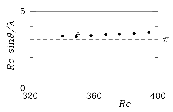
Right: Plot of as a function of Re for the experimentally observed patterns of Prigent et al. (Prigent et al. 2003, Prigent & Dauchot 2005). The open triangle shows for the case studied numerically in this paper.
We believe that equation (48) provides a good first approximation for the relationship between Re, , and . Figure 28 (right) shows a plot of as a function of Re from the experimental data of Prigent et al. (Prigent et al. 2003). It can be seen that this combination of quantities is approximately constant with a value near . The range of values of the individual factors Re, , and can be seen in table 3. In prior studies Barkley & Tuckerman 2005a; Barkley & Tuckerman 2005b, we have studied a large range of Reynolds numbers and tilt angles in a domain of length . In this domain, the wavelength of a periodic pattern is less constrained, though it must be a divisor of 120. Figure 29 shows the observed states as a function of Re and . Equation (48) captures the correct order of magnitude of ; specifically . Moreover, in figure 29 one sees that for fixed , increases with increasing , as (48) predicts.
Equation (48) does not hold in detail, however. Most notably, figure 29 shows that when is decreased at fixed , the wavelength increases rather than decreases as one would expect from (48). We believe that the force balance (15) holds for all patterns which possess a laminar region free of turbulence, but that the additional approximations made in deriving the simple relationship (48) do not hold over the full range of conditions considered in figure 29. In particular, the right-hand-side of (47) depends implicitly on , , and via the dependence of , , and on these quantities. The approximate functional relationships between , and that we have observed in our simulations and on which we have relied in deriving (48) may not hold for other parameter values. Finer adjustments must come from another mechanism.

The main issue not addressed in our study is closure. We have not attempted to relate the forcing of the mean flow due to Reynolds stresses back to the mean flow itself. In the future we will report on studies employing closure models.
Acknowledgements.
We thank F. Daviaud, O. Dauchot, P. Le Gal, P. Manneville and A. Prigent for helpful comments. The simulations analyzed in this work were performed on the IBM Power 4 of the IDRIS-CNRS supercomputing center as part of project 1119. This work was supported in part by a CNRS-Royal Society grant. \oneappendix5 Turbulent-laminar bands in other shear flows
| PC | TC | RS | PP | ||||
|---|---|---|---|---|---|---|---|
| 340 | 395 | 340 | 415 | 303 | 438 | 357 | |
| 110 | 110 | 145 | 95 | 71 | 106 | 103 | |
| 83 | 52 | 70 | 35 | 24 | 36 | 45 | |
| 60 | 46 | 63 | 33 | 23 | 34 | 41 | |
Turbulent-laminar banded patterns have been observed in a number of shear flows: plane Couette (PC) flow, Taylor-Couette (TC) flow, rotor-stator (RS) flow (torsional Couette flow; the flow between differentially rotating disks) and plane Poiseuille (PP) flow (channel flow). Comparisons between these flows are impeded by the fact that different conventions are used to non-dimensionalise each of them.
In order to compare their observations in Taylor-Couette flow with those in plane Couette flow, Prigent et al. 2003 generalise the Reynolds number used in plane Couette flow by considering it as based on the shear and the half-gap:
| (49) |
For flows whose shear is not constant, the average shear is used. We also convert streamwise and spanwise wavelengths to total wavelength and angle of the pattern wavevector via
| (50) |
Table 3 presents the Reynolds numbers, wavelengths, and angles for which turbulent-laminar patterns have been observed experimentally or numerically. The subsections which follow explain how Table 3 was obtained from the data in Prigent et al. 2003; Cros & Le Gal 2002; Tsukahara et al. 2005.
5.1 Taylor-Couette flow
For Taylor-Couette flow between differentially rotating cylinders, the azimuthal and axial directions correspond to the streamwise and spanwise directions of plane Couette flow. For cylinders of radius and , rotating at angular velocities and with and , the shear averaged over the gap is
| (51) |
leading to the Reynolds number:
| (52) |
where the last approximate equality corresponds to exact counter-rotation () and the narrow gap limit (), and , are the conventionally defined inner and outer Reynolds numbers, e.g. . The wavelengths and Reynolds numbers observed in Taylor-Couette and plane Couette flow are compared in Figure 5 of Prigent et al. 2003.
5.2 Torsional Couette flow
The laminar profile for torsional Couette flow between a rotating and a stationary disk (rotor-stator flow) is
| (53) |
and the Reynolds number based on axial shear and half-gap is
| (54) |
For spirals, the azimuthal wavelength in units of the half-gap is
| (55) |
Turbulent spiral patterns which are rather regular occur for a range of angular velocities and radii. In their figures 12, 16 and 18, Cros & Le Gal 2002 focus particularly on the radius and gap:
| (56) |
The highest and lowest rotation rates for which turbulent spirals are seen are
{subeqnarray}
ω= 68 rev/min =
7.12 rad/sec with m=6
ω= 47 rev/min =
4.92 rad/sec with m=9
Substituting (56)-(5.2) and the viscosity
cm2/sec of water into (54)-(55)
leads to the values shown in Table 3. The pitch angle of the
spirals remains approximately constant at . We use
(50) to calculate and ,
neglecting the variation in radius.
5.3 Plane Poiseuille flow
Figure 14 of Tsukahara et al. 2005 shows a visualisation from a direct numerical simulation of plane Poiseuille (PP) flow in a channel with domain and Reynolds number
| (57) |
where is the centerline velocity. The domain contains a single wavelength of an oblique turbulent-laminar banded pattern oriented at to the streamwise direction. (Both the wavelength and the angle are dictated by the computational domain.) Following Waleffe 2003, we view the Poiseuille profile in the half-channel , over which the shear has one sign, as comparable to the Couette profile in the channel , and thus take as the unit of length, rather than . The shear is obtained by averaging over :
| (58) |
For the Reynolds number based on the average shear and half-gap, we obtain
| (59) |
References
- Andereck et al. (1986) Andereck, C. D., Liu, S. S. & Swinney, H. L. 1986 Flow regimes in a circular Couette system with independently rotating cylinders. J. Fluid Mech. 164, 155–183.
- van Atta (1966) van Atta, C. W. 1966 Exploratory measurements in spiral turbulence. J. Fluid Mech. 25, 495–512.
- Barkley & Tuckerman (2005a) Barkley, D. & Tuckerman, L. S. 2005a Computational study of turbulent laminar patterns in Couette flow. Phys. Rev. Lett. 94, 014502.
- Barkley & Tuckerman (2005b) Barkley, D. & Tuckerman, L. S. 2005b Turbulent-laminar patterns in plane Couette flow. In IUTAM Symposium on Laminar-Turbulent Transition and Finite Amplitude Solutions (ed. T. Mullin & R. Kerswell), pp. 107–127. Dordecht: Springer.
- Bottin et al. (1998) Bottin, S., Daviaud, F., Manneville, P. & Dauchot, O. 1998 Discontinuous transition to spatiotemporal intermittency in plane Couette flow. Europhys. Lett. 43, 171–176.
- Coles (1965) Coles, D. 1965 Transition in circular Couette flow. J. Fluid Mech. 21, 385–425.
- Coles & van Atta (1966) Coles, D. & van Atta, C. W. 1966 Progress report on a digital experiment in spiral turbulence. AIAA J. 4, 1969–1971.
- Crawford & Knobloch (1991) Crawford, J. & Knobloch, E. 1991 Symmetry and symmetry-breaking bifurcations in fluid dynamics. Annu. Rev. Fluid Mech. 23, 341–387.
- Cros & Le Gal (2002) Cros, A. & Le Gal, P. 2002 Spatiotemporal intermittency in the torsional Couette flow between a rotating and a stationary disk. Phys. Fluids 14 (11), 3755–3765.
- Dauchot & Vioujard (2000) Dauchot, O. & Vioujard, N. 2000 Phase space analysis of a dynamical model for the subcritical transition to turbulence in plane Couette flow. Eur. Phys. J. B 14, 377–381.
- Eckhardt & Mersmann (1999) Eckhardt, B. & Mersmann, A. 1999 Transition to turbulence in a shear flow. Phys. Rev. E 60, 509–517.
- Hamilton et al. (1995) Hamilton, J. M., Kim, J. & Waleffe, F. 1995 Regeneration mechanisms of near-wall turbulence structures. J. Fluid Mech. 287, 317–348.
- Hegseth et al. (1989) Hegseth, J. J., Andereck, C. D., Hayot, F. & Pomeau, Y. 1989 Spiral turbulence and phase dynamics. Phys. Rev. Lett. 62 (3), 257–260.
- Henderson & Karniadakis (1995) Henderson, R. D. & Karniadakis, G. E. 1995 Unstructured spectral element methods for simulation of turbulent flows. J. Comput. Phys. 122 (2), 191–217.
- Jiménez & Moin (1991) Jiménez, J. & Moin, P. 1991 The minimal flow unit in near-wall turbulence. J. Fluid Mech. 225, 213–240.
- Lagha & Manneville (2006) Lagha, M. & Manneville, P. 2006 On the modeling of transitional plane Couette flow. Eur. Phys. J. B to appear.
- Manneville & Locher (2000) Manneville, P. & Locher, F. 2000 A model for transitional plane Couette flow. C.R. Acad. Sci. Paris II b 328, 159–164.
- Moehlis et al. (2004) Moehlis, J., Faisst, H. & Eckhardt, B. 2004 A low-dimensional model for turbulent shear flows. NJP 6, 56.
- Moehlis et al. (2002) Moehlis, J., Smith, T. & Holmes, P. 2002 Models for turbulent plane Couette flow using the proper orthogonal decomposition. PF 14, 2493–2507.
- Pope (2000) Pope, S. 2000 Turbulent Flows. Cambridge: Cambridge University Press.
- Prigent & Dauchot (2000) Prigent, A. & Dauchot, O. 2000 ’Barber pole turbulence’ in large aspect ratio Taylor-Couette flow. arXiv:cond-mat/00009241 .
- Prigent & Dauchot (2005) Prigent, A. & Dauchot, O. 2005 Transition to versus from turbulence in subcritical Couette flows. In IUTAM Symposium on Laminar-Turbulent Transition and Finite Amplitude Solutions (ed. T. Mullin & R. Kerswell), pp. 193–217. Dordecht: Springer.
- Prigent et al. (2003) Prigent, A., Gregoire, G., Chaté, H. & Dauchot, O. 2003 Long-wavelength modulation of turbulent shear flows. Physica D174 (1-4), 100–113.
- Prigent et al. (2002) Prigent, A., Gregoire, G., Chaté, H., Dauchot, O. & van Saarloos, W. 2002 Large-scale finite-wavelength modulation within turbulent shear flows. Phys. Rev. Lett. 89 (1), 014501.
- Schmiegel & Eckhardt (1997) Schmiegel, A. & Eckhardt, B. 1997 Fractal stability border in plane Couette flow. Phys. Rev. Lett. 79 (26), 5250.
- Smith et al. (2005) Smith, T., Moehlis, J. & Holmes, P. 2005 Low-dimensional models for turbulent plane Couette flow in a minimal flow unit. J. Fluid Mech. 538, 71–110.
- Tsukahara et al. (2005) Tsukahara, T., Seki, Y., Kawamura, H. & Tochio, D. 2005 DNS of turbulent channel flow at very low Reynolds numbers. In Proc. 4th Int. Symp. on Turbulence and Shear Flow Phenomena, pp. 935–940.
- Waleffe (1997) Waleffe, F. 1997 On a self-sustaining process in shear flows. Phys. Fluids 9 (6), 883–900.
- Waleffe (2003) Waleffe, F. 2003 Homotopy of exact coherent structures in plane shear flows. Phys. Fluids 15 (6), 1517–1534.