Stability properties of the collective stationary motion of self-propelling particles with conservative kinematic constraints
Abstract
In our previous papers we proposed a continuum model for the dynamics of the systems of self-propelling particles with conservative kinematic constraints on the velocities. We have determined a class of stationary solutions of this hydrodynamic model and have shown that two types of stationary flow, linear and radially symmetric (vortical) flow, are possible. In this paper we consider the stability properties of these stationary flows. We show, using a linear stability analysis, that the linear solutions are neutrally stable with respect to the imposed velocity and density perturbations. A similar analysis of the stability of the vortical solution is found to be not conclusive.
V.I. Ratushnaya1, D. Bedeaux1,2, V.L. Kulinskii3, A.V.
Zvelindovsky4
1Colloid and Interface Science group, LIC, Leiden University,
P.O. Box 9502, 2300 RA Leiden, The Netherlands
2Department of
Chemistry, Norwegian University of Science and Technology, 7491
Trondheim, Norway
3Department for
Theoretical Physics, Odessa National University, Dvoryanskaya 2,
65026 Odessa, Ukraine
4Department of Physics, Astronomy &
Mathematics, University of Central Lancashire, Preston PR1 2HE,
United Kingdom
PACS. 05.65.+b - Self-organized systems.
PACS. 47.32.-y - Rotational flow and vorticity.
PACS. 87.10.+e - General theory and mathematical aspects.
1 Introduction
The dynamics of the systems of self-propelling particles (SPP) is of a great interest for physicists as well as for biologists because of the complex and fascinating phenomenon of the emergence of the ordered motion. In nature these systems are represented by flocks of birds, schools of fishes, groups of bacteria etc. [1]-[3]. From the physical point of view many aspects of the observed non-equilibrium phase transition from disordered to ordered motion are to a large extent still an open problem.
The first numerical model simulating the behavior of the SPP was proposed by T. Vicsek at al. [4]. Their model is based on a kinematic rule imposed on the orientations of the velocities of the self-propelling particles. At a low noise amplitude and a high density it was shown that the system undergoes the transition from the disordered state to coherent motion. The nature of the transition is not established yet. T. Vicsek’s investigation shows that the occurring transition is of the second order. Several extensions of T. Vicsek’s model have been proposed, which consider particles with varying velocities, different types of noise, and including external force fields and/or interparticle attractive and repulsive forces [5]-[7]. The simulations performed in [7] show the discontinuous nature of the transition in the T.Vicsek’s model.
Properties of T. Vicsek’s model were also investigated analytically. In [8] the spontaneous emergence of ordered motion has been studied in terms of so-called control laws, using graph theory. Generalizations of the control laws were considered in [9, 10]. In [10] it was shown that the organized motion of SPP with the control laws depending on the relative orientations of the velocities and relative spacing, can be of two types only: parallel and circular motion. The stability properties of these discrete updating rules (including the T.Vicsek’s model) and the dynamics they describe were considered using Lyapunov theory in [8, 9, 11].
In our first paper [12] we constructed a hydrodynamic model for the system of self-propelling particles with conservative kinematic constraints, which can be considered as a continuum analogue of the discrete dynamic automaton proposed by T. Vicsek et al.
Based on the conservation of the kinetic energy and the number of particles our model is represented by the following equations:
| (1) | |||||
| (2) |
where and are the velocity and the density fields respectively and is an angular velocity field which takes into account the non-potential character of the interactions between the particles. We modeled this field as follows:
| (3) | |||||
where are the averaging kernels. In particular we considered a simple case of averaging kernels:
| (4) |
We call this the local hydrodynamic model (LHM). In this case Eq. (3) reduces to
| (5) |
where
| (6) |
In our second article [13] we have shown that the only regimes of the stationary planar motion in our model are either of translational or axial symmetry. In this respect our continuum model gives results similar with those obtained in the discrete model of T.Vicsek [4, 5].
In this paper we investigate the stability of the obtained regimes of motion with respect to small perturbations. In the next section we consider the stability of the planar stationary linear flow with respect to the velocity perturbation directed along the stationary flow and perpendicular to the flow. We show that in both cases the evolution of the perturbations has an oscillatory behavior, which means that they neither grow nor decay with time. This can be interpreted as neutral stability [14] of the corresponding stationary flow. Also the external pressure term can be included into Eq. (1) in order to account for potential external forces. In such a case with there exists the special case of the incompressible flows, , when the equations of motion coincide with that for potential flow of ideal fluids. As is known [14] such motion in geometry is stable in the Lyapunov sense.
In the third section we consider the stability of the planar stationary radially symmetric (vortical) motion of SPP with constant velocity and the density. We find that in this case the linear analysis does not lead to a conclusive answer about the stability of the solution.
2 Stability of planar stationary linear flow in the local hydrodynamic model
2.1 Stability with respect to a velocity perturbation along the flow
In this section we consider the stability properties of planar stationary linear flow for the local hydrodynamic model with , which we further call local hydrodynamic model 1 (LHM1). At the end of the section we will shortly discuss how these results extend to the local hydrodynamic models with and . For LHM1 the stationary linear flow is given by
| (7) |
where and are constants.
We consider velocity and the density perturbations of the following form:
| (8) |
The velocity perturbation chosen is directed along the stationary linear flow. Here are constants, is the wave vector and is an exponent, which determines the time evolution of the perturbation.
Substituting the solution into Eqs. (1)-(2) we obtain the linearized system of equations:
| (9) | |||||
| (10) |
For the perturbation (8) this system reduces to
| (11) | |||||
| (12) | |||||
| (13) |
Using Eq. (8) one may obtain the relation between and the wave number. From Eq. (11) it follows that
| (14) |
whereas from the linearized continuity equation (13) we have
Both the equalities are satisfied only in the case when .
Thus, in the linear stability analysis with respect to small deviations of the velocity and density fields, we obtain the following perturbed solution
| (15) |
Taking the real part of the density perturbation we have
| (16) |
The corresponding density field is shown on Fig1.
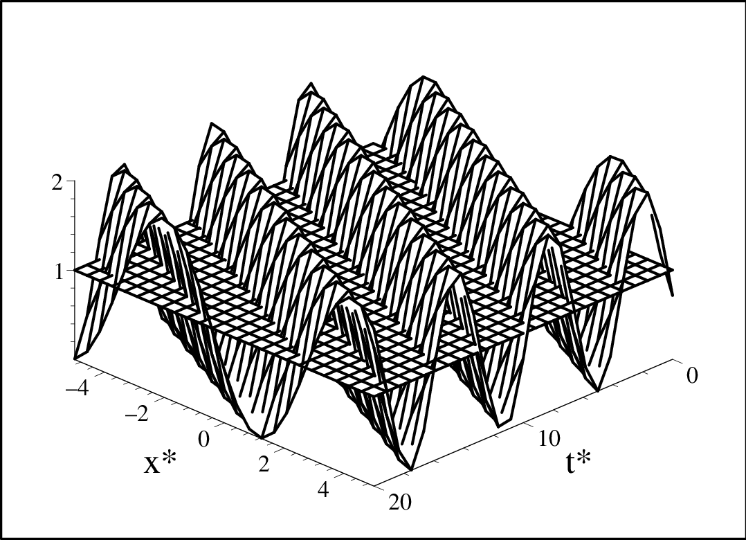
This flow Eq. (16) should satisfy the linearized system of the constraints (conservation of the kinetic energy and the number of particles) which are imposed on any solution of our model. This implies that the following conditions must be fulfilled:
| (17) | |||||
| (18) |
Since both conditions reduce to
| (19) |
If one integrates Eq. 19 over the period of the integrand, one may can that this condition is fulfilled.
The obtained perturbed flow is an oscillatory field (perturbation oscillates with a frequency as ) which means that the corresponding stationary solution is neither stable nor unstable within the first order perturbation theory. In other words we may conclude that in our local hydrodynamic model the stationary linear flow is neutrally stable with respect to a small density field perturbations.
The stability analysis of the other possible hydrodynamic models with or gives qualitatively similar result.
2.2 Stability with respect to a velocity perturbation perpendicular to the flow
In this section we investigate the stability properties of the stationary linear flow in the LHM1, Eq. (7), with respect to a velocity perturbation normal to the stationary flow. We consider only a velocity perturbation, which we take in the form of a plane wave:
| (20) |
where is a constant, is a wave vector and the exponent describes the time evolution of the perturbation.
Substituting the perturbation in the linearised equations (9)-(10) it follows that
| (21) | |||||
| (22) |
which imply that
| (23) |
Thus the time evolution of the perturbed velocity field is determined by the purely imaginary exponent in Eq. (23):
| (24) |
where the ”phase speed” is given by
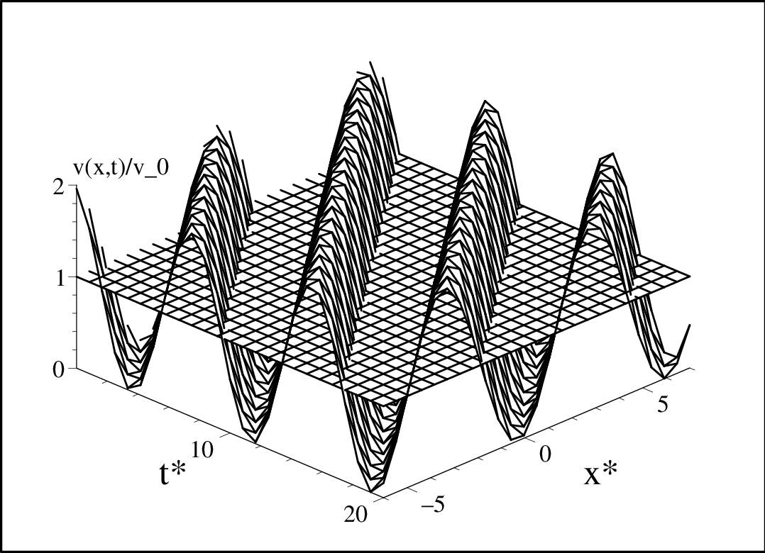
Taking the real part of the velocity perturbation we obtain as final result:
| (25) |
The corresponding velocity profile is shown in Fig.2.
Since the velocity perturbation was taken to be normal to the unperturbed field and , both of the constraints of the constancy of the kinetic energy and the number of particles, Eqs. (17)-(18), are satisfied.
As one may see the time dependent part of the velocity perturbation is a finite oscillatory function which means that the corresponding stationary solution is neutrally stable.
As in the previous section the stability analysis of the other possible hydrodynamic models with or gives qualitatively similar result.
3 Stability of stationary vortical flow with constant velocity and density in the local hydrodynamic model
As we have shown in our previous article [13] there are two classes of the stationary flows in the LHM, linear and radially symmetric or vortical flow.
The stationary vortical solution of the LHM1 () is given by , [12], where
| (26) |
Here is a cut-off radius of the vortex core and the constant is detemined by the circulation of the core
| (27) |
We consider small perturbations of the velocity field and of the density field. The linearized system in the LHM1 is then given by
| (28) | |||||
| (29) |
In this section we consider the stability of a particular class of stationary vortical flow for which the density is constant and given by . Substitution in Eq. (26) results in a constant velocity field . We write the small perturbation in the general form
| (30) |
For the projections of the velocity field together with the continuity equation for the density field we have
| (31) | |||||
| (32) | |||||
| (33) |
In order to simplify the problem we restrict our discussion to the case with the radial component of the velocity perturbation being constant, i.e. .
Then one can transform equations (31)-(33) into
| (34) | |||||
| (35) | |||||
| (36) |
The velocity perturbation must be a periodic functions of the angle and can therefore be written as:
| (37) |
where is a function of , is an integer and is a constant factor, which describes the time evolution of the perturbation, Eq. (30). Substituting this into Eq. (34) one obtains
| (38) |
and consequently
| (39) |
From Eq. (35) it follows that
| (40) |
Substituting this into Eq. (36) we obtain that .
The solutions (39) and (40) satisfy the linearized system of constraints, Eqs. (17) and (18), as one can see by angular integration.
Thus, we see that the time evolution of the perturbation Eq. (30) is determined by the purely imaginary exponent Eq. (38).
As a result the whole solution for the velocity and the density profiles has the following form:
| (43) | |||||
| (44) | |||||
The velocity field is shown in Fig. 3 for and .
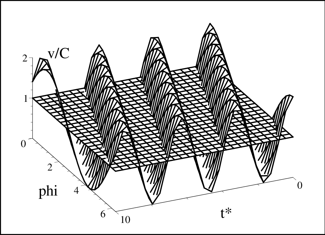
Together with the oscillatory contributions we now also have the contribution proportional to times an oscillating function. This does not necessarily mean that the stationary vortical flow is unstable. The obtained result indicates that the linear analysis does not give a definite answer regarding the stability of the stationary flow. The linear analysis does not give the definitive answer regarding the stability of the stationary flow and further investigation of higher order terms is required. This is beyond the scope of the present paper.
4 Conclusions
In this paper we considered the stability properties of the planar stationary flows of the local hydrodynamic model constructed in our first paper for a system of self-propelling particles [12]. These flows are the linear flow and the radially symmetric flow. Our analysis shows for linear flow, using linear perturbation theory, that the time evolution of the imposed velocity and density perturbations are oscillatory. It follows that the linear flows are neutrally stable. For radially symmetric (vortical) flow linear perturbation theory does not lead to a conclusive result. A definitive answer about the nature of the stability can only be given by considering also higher order terms in the perturbation expansion. Such an analysis is beyond the scope of the present paper. Note that such a situation is typical for Hamiltonian systems which are conservative by definition and therefore do not display an asymptotic type of stability [14].
References
- [1] Camazine S, Deneubourg J-L, Franks N R, Sneyd J, Theraulaz G, Bonabeau E 2001 Self-Ogranization in Biological Systems (Princeton and Oxford: Princeton University Press)
- [2] Parrish J K, Hamner W M 1997 Three dimensional animals groups (Cambridge: Cambridge University Press)
- [3]
Parrish J K, Edelstein-Keshet L 1999 Science 284
99
Parrish J K, Viscido S V, Grnbaum D 2002 Biol. Bull. 202 296 - [4]
Vicsek T, Czirók A, Ben-Jacob E, Cohen I, Shochet O 1995
Phys. Rev. Lett. 75 1226
Czirók A, Stanley H E, Vicsek T 1997 J. Phys. A: Math. Gen. 30 1375 - [5] Czirók A, Ben-Jacob E, Cohen I and Vicsek T 1996 Phys. Rev. E 54 1791
- [6] Hubbard S, Babak P, Sigurdsson S Th, Magnússon K G 2004 Ecological Modelling 174 359
- [7]
Grégoire G, Chaté H 2004 Phys. Rev. Lett.
92 025702
Grégoire G, Chaté H, Tu Y 2003 Physica D 181 157 - [8] Tanner H G, Jadbabaie A, Pappas G J 2005 Cooperative control lecture notes in control and information sciences 309 229
- [9] Jadbabaie A, Lin J, Morse A S 2003 IEEE transactions on automatic control 48 988
- [10] Sepulchre R, Paley D, Leonard N 2005 Cooperative control lecture notes in control and information sciences 309 189
- [11]
Gazi V, Passino K M 2003 IEEE transactions on automatic
control 48 692
Gazi V, Passino K M 2004 IEEE transactions on systems, man, and cybernetics - part B: cybernetics 34 539 - [12] Kulinskii V, Ratushnaya V, Zvelindovsky A, Bedeaux D 2005 Europhys. Lett. 71 207
- [13] Ratushnaya V, Kulinskii V, Zvelindovsky A, Bedeaux D 2006 Physica A 366 107
- [14] Arnold V I 1978 Mathematical Methods of Classical Mechanics (New York, NY: Springer)