Maximum Likelihood Estimation of Drift and Diffusion Functions
Abstract
The maximum likelihood approach is adapted to the problem of estimation of drift and diffusion functions of stochastic processes from measured time series. We reconcile a previously devised iterative procedure Kleinhans05 and put the application of the method on a firm theoretical basis.
Keywords:
Nonlinear time series analysis, Diffusion process, Sparsely sampled datapacs
05.10.Gg, 05.45.TpI Introduction
Complex systems of physics, chemistry, and biology are composed of a huge number of microscopic subsystems interacting on a fast time scale. Self organized behaviour may arise on a macroscopic length and time scale which can be described by suitably defined order parameters. The microscopic degree’s of freedom, however, show up in terms of fast temporal variations which effectively can be treated as random fluctuations Haken:Synergetics. The adequate description of such systems viewed from a macroscopic perspective are Langevin equations, which contain a deterministic part described by the drift vector and a fluctuating part whose impact on the dynamics is quantified by a diffusion matrix Risken; Gardiner.
Recently, a procedure has been proposed that allows for a direct estimation of these quantities and, hence, of the stochastic dynamics from measured data Siegert98. This procedure has provided a deeper insight to a broad class of systems, especially in the field of life sciences Kriso02; Siegert98; Kuusela04. Moreover, also turbulence research has greatly benefited from this procedure Friedrich97.
However, the procedure is based on the estimation of conditional moments in the limit of high sampling frequencies,
| (1) |
for and , respectively. is the drift vector, while exhibits the diffusion matrix of the underlying process at position . The limiting procedure (1) can be problematic in case of a finite time resolution of measured data. Moreover, any presence of measurement or discretization noise seriously interferes with the convergence of the limiting procedure 11 1 The application of this procedure in presence of measurement noise recently has been investigated, see Boettcher06..
Recently, we proposed an iterative method that circumvents this limiting procedure Kleinhans05. It is based on the minimization of the Kullback-Leibler distance Haken:Information; Kullback between the two time joint probability distribution functions (pdf) obtained from the data and the simulated process for a certain set of parameters, respectively. The starting configuration of this iterative procedure as well as a suitable parametrization of drift and diffusion functions can be obtained by the direct estimates based on the smallest reliable time increment , provided by (1).
On the other hand, the analysis of discrete stochastic processes by means of maximum likelihood-methods has made great progress in recent years: Since it has become evident, that the maximisation of the likelihood function is a powerful tool for the analysis of Markovian time series Lo88, several methods have been proposed to optimise the calculation of the required conditional transition pdfs Sahalia02; Nicolau02. For a recent study on the preferences of current methods we refer to Hurn03.
The intention of the present note is to derive a maximum likelihood estimator for parameters of the parametrized drift vector and diffusion matrix, that purely is based on the conditional and joint transition pdfs of the dataset under consideration. By this means, the Kullback-Leibler estimator reappears in case of an ensemble of individual measurements – but now physically well motivated. We want to point out, that the evaluation of a specific parametrisation by means of the minimization of the Kullback-Leibler estimator yields great advantages, since this function is bounded from below by the value . Hence, the goodness of a single parametrisation can be assessed.
Moreover, with respect to our previous treatment Kleinhans05, a simplified maximum likelihood estimator is introduced for the analysis of nonlinear time series exhibiting Markovian properties. This estimator leads to a reasonable reduction of the required computational effort compared to a direct application of the former method and is proposed for future application in nonlinear time series analysis. Accurate results can be obtained even in the case of few or sparsely sampled measurement data. However, the relevance of the results obtained in the case of data sets involving few data points carefully has to be reconsidered in a self consistent manner.
II Maximum Likelihood Estimation on Ensembles: Reconciliation with the Kullback-Leibler estimator Kleinhans05
We consider time series , of recordings of a multivariate stochastic variable. Furthermore, we assume that the time lag between consecutive observations is . Henceforth, the abbreviation will be used.
In this section, the estimation of drift and diffusion functions from an ensemble of independent time series is considered. Such data sets generally are obtained from measurements on an ensemble of independent systems, that are performed simultaneously. In this vein, the time evolution of the stochastic properties can be analysed. For the present case, we restrict ourselves without loss of generality to the analysis of the first two consecutive measurements and with .
By means of the direct estimation described in Siegert98, drift and diffusion functions can be estimated from data from the Kramers-Moyal expansion coefficients (1). On the basis of this estimate, models for the drift and diffusion function, respectively, can be constructed, depending on a set of parameters, . This procedure is described in greater detail in Kleinhans05.
The likelihood of the current realization for one specific set of parameters, , can be expressed by means of the joint pdf,
| (2) |
Since the individual processes are assumed to be statistically independent of one another, this joint pdf degenerates into a product of two point joint pdfs,
| (3) |
This expression can be simplified considerably.
First, we consider the logarithm of (3), usually called log-likelihood function Kalbfleisch:II,
| (4) |
With help of expression (4) finally can be evaluated by means of an integral,
| (5) | |||
Since the logarithm is a monotonically increasing function, the maximization of the likelihood function is equivalent to the maximization of its logarithm. The set , that maximizes the latter expression, therefore forms the most likely set of parameters under the current parametrization.
In Kleinhans05, for the present case the minimization of the Kullback distance of the joint distributions has been proposed,
III Maximum Likelihood estimation on Markovian time series
Henceforth, individual time series are considered. We assume that the time lag between consecutive observations is and that the process is stationary in a sense, that the statistical properties are conserved during the measurement period.
Let us further assume, that the data set under consideration exhibits Markovian properties. This can be verified by means of the Chapman-Kolmogorov equation Risken; Gardiner,
| (7) |
that can be evaluated numerically. Although this condition is not sufficient, it seems to be a very robust criterion. If Markovian properties are not fulfilled, an increase of the number of observables by means of a delay embedding of the data may help to fulfil this constraint, if the amount of data is sufficiently high for such an procedure Risken.
If the process under consideration is ergodic, time averages can be evaluated by means of ensemble averages. Then, also in this case a reasonable parametrization and initial condition for the vector can be obtained by the direct evaluation of (1), as described in the previous section. Let us now iterate the arguments of the previous section.
The likelihood of the current realization for a specific set of parameters, , is
| (8) |
Since we assume Markov properties, this joint pdf degenerates into a product of two point conditional pdfs,
| (9) |
This expression can be simplified by considering the logarithm of the likelihood function. With the help of the definition
| (10) |
we finally obtain:
| (11) | |||
Following the maximum likelihood approach, this expression has to be maximized with respect to . This is consistent with the minimization of
| (12) | |||||
It is obvious, that in the latter expression the first summand is negligible for . Even in the case of smaller , the first measurement in some cases may not obey the stationary distribution due to transient processes of the measurement. On the other hand, the evaluation of the expression may be time-consuming since the stationary distribution of the process is required. In conclusion, we propose to solely perform the minimization of
| (13) |
IV Minimization Procedure for Drift-/Diffusion-Processes
We would like to emphasize, that expression (13) can be evaluated numerically. It is a feature of drift and diffusion processes, that the time evolution of the conditional pdf can be obtained from the Fokker-Planck equation Risken,
| (14) | |||
This equation can be treated efficiently by implicit algorithms at least for the case and , respectively NrFortran. Moreover, kernel density estimates based on numerical integration of the associated stochastic differential equation can be applied, that are described in greater detail in Hurn03.
The data under consideration can be reduced significantly by a suitable discretization of data space in several bins. Typically, this grid should coincidence with the spatial discretization required for numerical solution of the Fokker-Planck equation. After discretization and numerical evaluation of the expression , equation (13) can be evaluated my means of a finite sum.
Eventually, the set , that minimizes (13) has to be investigated. This can be done by gradient method or more efficient approaches NrFortran. We want to emphasize that in the majority of cases a suitable starting value is obtained from the initial estimates (1). This is essential for a successful and fast minimization by any numerical algorithm.
V Example
In this section, the performance of the minimization procedure is discussed by means of an example, that can be treated analytically. Further examples of the minimization procedure are investigated in Kleinhans05; Nawroth07 for numerical and experimental data, respectively.
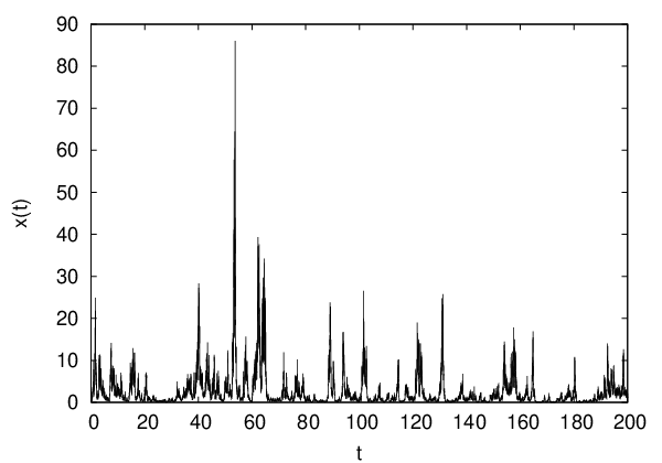
| We would like to address a drift and diffusion process in one dimension with the diffusion term | |||
| (15a) | |||
| that in the long term limit obeys a lognormal distribution | |||
| (15b) | |||
| This complies with the drift function | |||
| (15c) | |||
| Thus, a stochastic process with a nonlinear drift term is discussed, that is driven by multiplicative dynamical noise. A feasible path of this process can be obtained by numerical integration of the associated stochastic differential equation. A sample graph of the process is exhibited in figure 1. Thereby, Itô’s interpretation of stochastic differential equations (sde) was applied. For the detailed properties of drift and diffusion processes we refer to Risken. | |||
For any one-dimensional process, the diffusion term significantly can be simplified by means of a nonlinear transformation of the state variable: For
| (16) |
the drift and diffusion functions transform to Risken
| (17a) | |||||
| (17b) | |||||
In the present case, the accordant nonlinear transformation and the transformed drift and diffusion functions are:
| (18a) | |||||
| (18b) | |||||
| (18c) | |||||
Hence, the process is equivalent to an Ornstein-Uhlenbeck process in the transformed variable . For this process, the conditional transition pdfs can be derived for finite time increment Risken:
| (19) | |||||
Let us now consider the determination of the intrinsic parameters and from time series data. Imagine, the conditional pdfs are known from time series data for a specific set of parameters , that was applied for numerical integration of the sde. This initial set will now be reconstructed by means of the most likely set . Following the argument of section III, the minimization of
| (20) | |||||
is sufficient for this purpose.
This expression can be calculated by means of the underlying Ornstein-Uhlenbeck process,
| (21) | |||||
As a first step, the logarithm can be evaluated for the specific conditional transition pdfs of the Orstein-Uhlenbeck process under consideration, (19). It turns out, that the solely is determined by the second order moments of and :
| (22) | |||||

Finally, a closed form for the function can be derived:
| (23) | |||||
For the initial set , this function is exhibited in figure 2. A distinct minimum at is evident, that complies with the initial set of parameters. In case of an application of the minimization procedure to real measurements, this minimum would have to be approached by means of gradient methods or advanced minimization algorithms NrFortran.
VI Conclusion
In conclusion, the likelihood functions of stochastic processes have been derived for two specific cases. First, ensembles of measurements on these processes were considered. In this connection, the iterative procedure proposed in Kleinhans05 has been approved and physically motivated.
Moreover, the maximum likelihood approach has been adapted to the needs of non-linear time series analysis. For the case of Markovian processes, an integral form of the estimator has been derived. A slight simplification of this estimator, equation (13), is purely based on two point conditional pdfs, that can be calculated numerically from the Fokker-Planck equation in case of drift and diffusion processes. The integral form of the estimator allows for the reduction of huge datasets to their conditional transition pdfs prior to the iterative analysis procedure.
Finally, the meaning of the optimal set of parameters, , that is obtained by application of the method described in Kleinhans05, has been made explicit on the basis of the maximum likelihood approach: It is the most likely set of parameters with respect to the current parametrization. As a consequence, the proposed procedure can be applied even to time series that suffer from sparse data points and that could not safely be processed by the former methods without this knowledge.
References
- (1) D. Kleinhans, R. Friedrich, A. Nawroth, and J. Peinke, Phys Lett A 346, 42 (2005).
- (2) H. Haken, Synergetics, Springer Series in Synergetics (Springer-Verlag, Berlin, 2004), pp. xvi+763, introduction and advanced topics, Reprint of the third (1983) edition [Synergetics] and the first (1983) edition [Advanced synergetics].
- (3) H. Risken, The Fokker-Planck equation, Vol. 18 of Springer Series in Synergetics, 2nd ed. (Springer-Verlag, Berlin, 1989), pp. xiv+472, methods of solution and applications.
- (4) C. W. Gardiner, Handbook of stochastic methods for physics, chemistry and the natural sciences, Vol. 13 of Springer Series in Synergetics, 3rd ed. (Springer-Verlag, Berlin, 2004), pp. xviii+415.
- (5) S. Siegert, R. Friedrich, and J. Peinke, Physics Letters A 243, 275 (1998).
- (6) S. Kriso, R. Friedrich, J. Peinke, and P. Wagner, Physics Letters A 299, 287 (2002).
- (7) T. Kuusela, Physical Review E 69, 031916 (2004).
- (8) R. Friedrich and J. Peinke, Phys. Rev. Lett. 78, 863 (1997).
- (9) H. Haken, Information and self-organization, Springer Series in Synergetics, 2nd ed. (Springer-Verlag, Berlin, 2000), pp. xiv+222, a macroscopic approach to complex systems.
- (10) S. Kullback, in Information Theory and Statistics, edited by W. A. Shewhart and S. S. Wilks (Wiley Publications in Statistics, 1959).
- (11) A. W. Lo, Econometric Theory 4, 231 (1988).
- (12) Y. Ait-Sahalia, Econometrica 70, 223 (2002).
- (13) J. Nicolau, The Econometrics Journal 5, 91 (2002).
- (14) A. S. Hurn, K. A. Lindsay, and V. L. Martin, Journal of Time Series Analysis 24, 45 (2003).
- (15) J. D. Kalbfleisch, Probability and Statistical Inference II. Statistical Inference (Springer, Berlin, 1985).
- (16) W. H. Press, S. A. Teukolsky, B. P. Flannery, and W. T. Vetterling, Numerical Recipes in FORTRAN: The Art of Scientific Computing (Cambridge University Press, New York, NY, USA, 1992).
- (17) A. Nawroth, J. Peinke, D. Kleinhans, and R. Friedrich, Improved estimation of Fokker-Planck equations through optimisation (in preparation).
- (18) F. Böttcher et al., Phys. Rev. Lett. 97, 090603 (2006).