A Low-Noise High-Density Alkali Metal Scalar Magnetometer
Abstract
We present an experimental and theoretical study of a scalar atomic magnetometer using an oscillating field-driven Zeeman resonance in a high-density optically-pumped potassium vapor. We describe an experimental implementation of an atomic gradiometer with a noise level below 10 fT Hz-1/2, fractional field sensitivity below Hz-1/2, and an active measurement volume of about 1.5 cm3. We show that the fundamental field sensitivity of a scalar magnetometer is determined by the rate of alkali-metal spin-exchange collisions even though the resonance linewidth can be made much smaller than the spin-exchange rate by pumping most atoms into a stretched spin state.
pacs
07.55.Ge,32.80 Bx,33.35+r,76.60-kI Introduction
High-density hot alkali-metal vapors are used in such vital metrology applications as atomic clocks Knappe et al. 2004 and magnetometers Groeger et al. 2005; Aleksandrov 1995; Budker et al. 2000. In these applications the resolution of frequency measurements of the hyperfine or Zeeman resonance can be improved by increasing the density of alkali-metal atoms until the resonance begins to broaden due to alkali-metal spin-exchange (SE) collisions. Such broadening can be completely eliminated for Zeeman resonances near zero magnetic field Happer and Tang 1977; Happer and Tam 1977; Allred et al. 2002. The broadening of the hyperfine and Zeeman resonances at a finite magnetic field can be reduced by optically pumping the atoms into a nearly fully polarized state Appelt et al. 1999; Y.-Y.Jau et al. 2004; Savukov et al. 2005. These techniques have been used to demonstrate clock resonance narrowing Y.-Y.Jau et al. 2004 and have led to significant improvement in the sensitivity of atomic magnetometers Kominis et al. 2003 and to their application for detection of magnetic fields from the brain Xia et al. 2006 and nuclear quadrupole resonance signals from explosives Lee et al. 2006. However, the effects of SE collisions on the fundamental sensitivity of magnetometers operating in a finite magnetic field and on atomic clocks have not been analyzed in detail. Here we study experimentally and theoretically the effects of SE collisions in an atomic magnetometer operating in geomagnetic field range. It was shown in Appelt et al. 1999; Y.-Y.Jau et al. 2004; Savukov et al. 2005 that in the limit of weak excitation the Zeeman and hyperfine resonance linewidths can be reduced from , where is the alkali-metal SE rate, to , where is the alkali-metal spin-destruction rate, by pumping most of the atoms into the stretched spin state with maximum angular momentum. Since for alkali-metal atoms (for example, for K atoms ), this technique can reduce the resonance linewidth by a factor of . However, the frequency measurement sensitivity depends not only on the linewidth but also on the amplitude of the spin precession signal, and the optimal sensitivity is obtained for an excitation amplitude that leads to appreciable rf broadening. In this paper, we study rf broadening in the presence of non-linear evolution due to SE collisions and find that the fundamental limit on sensitivity is determined by even when most atoms are pumped into the stretched spin state and the resonance linewidth is much narrower than . We derive a simple relationship for the ultimate sensitivity of a scalar alkali-metal magnetometer, which also applies qualitatively to atomic clocks. We find that the best field sensitivity that could be realized with a scalar alkali-metal magnetometer is approximately 0.6 fT/Hz1/2 for a measurement volume of 1 cm3.
Scalar magnetometers measure the Zeeman resonance frequency proportional to the absolute value of the magnetic field and can operate in Earth’s magnetic field. They are important in a number of practical applications, such as mineral exploration Nabighian et al. 2005, searches for archeological artifacts et al. 2004 and unexploded ordnance Nelson and McDonald 2001, as well as in fundamental physics experiments, such as searches for a CP-violating electric dipole moment Groeger et al. 2005. Some of these applications require magnetometers that can measure small ( fT) changes in geomagnetic-size fields with a fractional sensitivity of . Existing sensitive scalar magnetometers use large cells filled only with alkali-metal vapor and rely on a surface coating to reduce relaxation of atoms on the walls Aleksandrov 1995; Budker et al. 2000; Groeger et al. 2005. Here we use helium buffer gas to reduce diffusion of alkali atoms to the walls, which also allows independent measurements of the magnetic field at several locations in the same cell Kominis et al. 2003. We present direct measurements of the magnetic field sensitivity in a gradiometric configuration and demonstrate noise level below 10 fT in a T static field (1 part in ) using an active measurement volume cm3. A small active volume and the absence of delicate surface coatings opens the possibility of miniaturization and batch fabrication Schwindt et al. 2004 of ultra-sensitive magnetometers. The best previously-reported direct sensitivity measurement for a scalar magnetometer, using a comparison of two isotopes of Rb occupying the same volume , had Allan deviation that corresponds to sensitivity of 60 fT Hz-1/2 and fractional sensitivity of Hz-1/2 Alexandrov et al. 2004. Theoretical estimates of scalar magnetometer sensitivity based on photon shot noise level on the order of 1 fT Hz-1/2 have been reported in cells with cm3 Aleksandrov 1995; Budker et al. 2000.
We rely on a simple magnetometer arrangement using optical pumping with circularly-polarized light parallel to the static magnetic field , excitation of spin coherence with an oscillating transverse magnetic field , and detection of spin coherence by optical rotation of a probe beam orthogonal to the static field. RF broadening of magnetic resonance is usually described by the Bloch equations with phenomenological relaxation times and Abragam 1961. Since SE collisions generally cause nonlinear spin evolution, such a description only works for small spin polarization Bhaskar et al. 1981. To study the general case of large polarization and large rf broadening we performed measurements of resonance lineshapes in K vapor for a large range of SE rates, optical pumping rates, and rf excitation amplitudes. We also developed a program for numerical density matrix modeling of the system. To understand the fundamental limits of the magnetometer sensitivity, we derive an analytical result that gives an accurate description of magnetometer behavior in the regime , where is the optical pumping rate, applicable to high density alkali-metal magnetometers with high spin polarization. In the limit of high polarization, we find an implicit equation for the transverse spin relaxation that can be solved to calculate polarization as a function of rf field detuning and other parameters. In this limit, the system is well-described by the solutions to the familiar Bloch equations, with varying as a function of polarization and rf field de-tuning. This modified Bloch equation model reproduces the non-Lorentzian resonance lineshape from the full density matrix simulation and the experimental rf broadening data and allows us to set analytical limits on the magnetometer sensitivity. The same approach can also be easily applied to other alkali metal atoms with different nuclear spin values and to hyperfine clock transitions.
This paper is organized as follows: Sec. II describes the experimental setup and presents measurements of magnetic field sensitivity and other experimental parameters. Sec. III presents a theoretical description of the magnetometer signals. Sec. IV gives expressions for the fundamental sensitivity of the magnetometer and compares this theoretical result to our high-sensitivity magnetometer measurements.

II Experimental measurements
II.1 Measurement apparatus
The scalar magnetometer, diagrammed in Fig. 1, is built around a Pyrex cell containing potassium in natural abundance, 2.5 amg of 4He to slow atomic diffusion, and 60 Torr of N2 for quenching. For characterization, the cell was heated to varying temperatures using a hot air oven. For the most sensitive magnetometry measurements, the cell was heated with pairs of ohmic heaters (wire meander in Kapton sheet) oriented to cancel stray fields and driven at 27 kHz. A circularly polarized pump beam at the resonance polarizes the K atoms along the -direction. The component of atomic spin polarization is measured using optical rotation of a linearly-polarized beam as determined by a balanced polarimeter. Two-segment photodiodes were used on each arm of the polarimeter to make a gradiometer measurement. A constant bias field is applied parallel to the pump laser. An oscillating rf field is applied in the direction with its frequency tuned to the Zeeman resonance given by for potassium atoms. The polarimeter measurement is read through a lock-in amplifier, tuned to the rf frequency. The lock-in phase is adjusted to separate the resonance signal into symmetric (in-phase) absorption and antisymmetric (out-of-phase) dispersion components. Exactly on resonance the dispersive part of the signal crosses zero. The magnitude of the local field is determined by the frequency of this zero-crossing and changes in the dc magnetic field are registered as deviations from zero of the dispersive signal.
II.2 Noise measurements with a high sensitivity atomic magnetometer
Magnetometer noise is read on the dispersive component of the lock-in reading. The conversion of the voltage noise to magnetic field noise depends on the slope as a function of the magnetic field or frequency of the dispersion curve. The tunable parameters of the experiment were adjusted to maximize the dispersion curve slope. The pump beam (20–40 mW) was imaged on an area of roughly cm2 across the cell. A probe beam cross section of cm2 was defined by a mask with total power of 10 mW and the wavelength detuned by about 100 GHz from the resonance. After passing through the cell and the polarizing beam splitter the probe beam was imaged onto two-segment photodiodes. For the most sensitive measurements, the amplitude of the oscillating rf field was about 19 nT. Magnetic field sensitivity was measured for three values of : 1 T, 10 T, and 26 T. The cell was heated to approximately 150∘C, yielding an atomic density of cm-3.

The polarimeter signals were measured with a lock-in amplifier (Stanford Research Systems SR830 for 1 T and 10 T measurements, SR844 for the 26 T measurement). The lock-in internal reference generated the rf field and the time constant was set to 100 s. The resonance lineshapes obtained by varying the rf frequency are shown in Fig. 2. The pump power and rf amplitude are adjusted to optimize the slope of the dispersion signal for a given probe beam power. At the parameters that optimized the magnetometer sensitivity, the resonance curves are well-described by Lorentzian lineshapes with similar half-width at half maximum (HWHM) for absorptive and dispersive components of 220 Hz for 1 T and 10 T and 265 Hz for 26 T. The amplitude and width of the optical rotation signal was found to be nearly independent of the static magnetic field values over the range of our measurements. The field was generated using a custom current source, based on a mercury battery voltage reference and a FET input stage followed by a conventional op-amp or a transistor output stage Baracchino et al. 1997. The fractional current noise was less than Hz1/2 at 10 Hz, about 10 times better than from a Thorlabs LDC201 ULN current source. Low-frequency ( Hz) optical rotation noise was reduced by an order of magnitude by covering the optics with boxes to reduce air convection that causes beam steering. The oven and laser beams within the magnetic shields were enclosed in a glass vacuum chamber to eliminate air currents.
Probe beam position was adjusted to equalize the photodiode signals for the two polarimeters within . The gradiometer measurements reduced by more than an order of magnitude the noise from the current source as well as pump intensity and light shift noise. By applying a calibrated magnetic field gradient, we found the effective distance between the gradiometer channels to be mm, much larger than the K diffusion length in one relaxation time mm, so the two measurements are independent.

The magnetic field data were acquired from the dispersive lock-in signal for 100 sec with a sampling rate of 2 kHz. The FFT of the data was converted to a magnetic field noise spectrum using a frequency calibration of the dispersion slope and corrected for the finite bandwidth of the magnetometer. The bandwidth was found to be close to the Lorentzian HWHM for all values of . The magnetic noise spectra at 1 T and 10 T are shown in Fig. 3. At 1 T, single channel measurements were limited by lock-in phase noise, while at 10 T they were limited by current source noise. The noise in the difference of the two channels was limited almost entirely by photon shot noise at higher frequencies and reached below 14 fT/, corresponding to less than 10 fT/ for each individual magnetometer channels. With the pump beam blocked, the optical rotation noise reached the photon shot noise level. Low frequency noise was most likely due to remaining effects of convection. At 26 T, the gradiometer had a sensitivity of 29 fT/, limited by lock-in phase noise and imperfect balance between gradiometer channels.
II.3 Magnetic resonance measurements
To analyze the magnetometer behavior and predict the theoretical sensitivity of the device, we focus on the shape of the magnetic resonance curves. The basic behavior of the resonance signals can be understood using phenomenological Bloch equations (BE), which predict a Lorentzian resonance lineshape. Though the BE cannot describe the whole physics in the case of rapid spin-exchange collisions, they do provide a convenient phenomenological framework for qualitative understanding of the resonance lineshape including the effects of rf broadening. Using the rotating wave approximation, the solution of the BE (see, for example Abragam 1961) in a frame rotating about the -axis is:
| (1) | |||||
| (2) | |||||
| (3) |
Here we introduce the in-phase and out-of-phase components of the transverse polarization in the rotating frame and the longitudinal polarization . In the lab frame, we measure , and we tune the lock-in phase to separate the absorptive from the dispersive . and are constant phenomenological relaxation times, is the equilibrium polarization, is the amplitude of the excitation field in the rotating frame, given by in the lab frame. The detuning is the difference between the rf frequency and the resonant frequency , which is the Larmor frequency in the applied dc field . The dependencies of and on frequency are Lorentzian, with the HWHM
| (4) |
The increase in the width due to the presence of excitation field is the basic phenomenon of rf resonance broadening. The slope, at resonance, of the dispersive component of the signal is given by
| (5) |
The slope has a maximum at an excitation field :
| (6) |
The accuracy of the simple Bloch equation theory depends on the contribution of spin-exchange relaxation to the linewidth. If the temperature is low, then the broadening due to optical pumping can exceed SE broadening, and the Bloch equation theory will be quite accurate. Additionally, if spin polarization is low, SE broadening will not depend significantly on the polarization and the excitation field, so the transverse relaxation time will be almost constant; in this case the BE solution is also valid. However, we are primarily interested in the regime of high spin-exchange rate and high spin polarization, where the magnetometer is most sensitive.
To understand the effects of SE broadening, we compared the lineshape predicted from the BE to the measured resonance lineshape of the magnetometer signal at a frequency of 80 kHz. We recorded the magnetic resonance curves for different values of rf excitation amplitude, pump laser intensity, and cell temperature. We find that the lineshape of the resonance remains reasonably close to a Lorentzian and the in- and out-of-phase lock-in data from resonance measurements were fit to the absorptive and dispersive Lorentzian profiles, allowing for some mis-tuning of the lockin phase. It can be seen from the BE that relative amplitudes of absorptive and dispersive components can differ substantially from those expected from a complex Lorentzian in the regime of large rf broadening. Moreover, due to SE effects, the absorption and dispersion widths for the same experimental conditions can also differ. Thus, a total of five parameters were used for each resonant curve: the resonant frequency, and the respective amplitudes and widths of the absorptive and dispersive signal components. An example of the results for the resonance linewidths as a function of the magnitude of the rf field is shown in Fig. 4. It can be seen that rf broadening is greater than what is expected from the BE. Moreover, the absorptive and dispersive parts of the resonance have different widths as the rf amplitude in increased. These are signatures of the SE broadening that require modifications of the BE description.
In the regime of small rf broadening we verified that the absolute size of the lock-in signal is in agreement with Bloch equations. The optical rotation signal detected by the lock-in is given by
| (7) |
where is the optical dispersion profile of the resonance line with linewidth and oscillator strength , is the density of atoms, is the length of the cell in the direction of the probe beam, and cm is the classical electron radius. Here we take into account the fact that lock-in output measures the r.m.s. of an oscillating signal. The length is determined by the dimensions of polarized vapor illuminated with the pump beam. Near the edges of the cell the pump beam is distorted, reducing below the inner dimensions of the cell. We varied the width of the pump beam to find that the largest pump width for which the signal still increases is about 2 cm. For this value of the absolute signal size was in agreement with Bloch equations to within 15%. So the volume of the polarized atomic vapor participating in the measurement is about cm cm3.

II.4 Relaxation rates
A number of independent auxiliary measurements were preformed to find the relaxation rates of the alkali-metal spins to be used for detailed modeling of SE effects. Spin exchange and spin destruction rates can be determined by measuring the width of the Zeeman resonance in a very low field using low pump and probe laser intensity Allred et al. 2002. For these measurements, the magnetic field was perpendicular to the plane of the lasers and the pump laser intensity was modulated near the Zeeman resonance. The signal as a function of modulation frequency was fit to a sum of two Lorentzians taking into account the counter-rotating component of pump rate modulation Savukov and Romalis 2005. At low magnetic field, when the Zeeman frequency is much smaller than the SE rate, SE broadening depends quadratically on the magnetic field. The spin-destruction rate is obtained from extrapolation of the width to the zero-field limit. From these fits of the resonant frequency and linewidth we determined the spin-exchange rate and the spin-destruction rate (SD) , which are listed in Table 1 for the same cell at several temperatures. The error bars are estimated from fits to different sets of the data. In addition, we determined the density of K atoms by scanning the DFB probe laser across the the optical absorption profile of the D1 resonance. The alkali densities calculated from the integral of the absorption cross-section using known oscillator strength () and cell length ( cm) are also shown in Table 1. The density is approximately a factor of 2 lower than the density of saturated K vapor at the corresponding temperature, as we find is common in Pyrex cells, probably due to slow reaction with glass walls. The alkali-metal SE rate can be calculated from the measured density using known K-K spin-exchange cross-section cm2 Alexandrov et al. 2002 and is in good agreement with direct measurements. The spin destruction rate can also be calculated using previously measured spin-destruction cross-sections for K-K, K-He and K-N2 collisions Chen et al. 2007 and gas composition in the cell (2.5 atm of 4He and 60 torr of N2). We also include relaxation due to diffusion to cell walls. Errors on the rates calculated from the densities are estimated from uncertainty in the cross-section and in the gas pressures in the cell. Our direct measurements of the spin-destruction rate are reasonably consistent with these calculations.
| Temp. | K density | ||||
|---|---|---|---|---|---|
| ∘C | s-1 | s-1 | ms-1 | ms-1 | 1012 cm-3 |
| 130 | 283 | 212 | 2.30.2 | 2.50.1 | 2.2 |
| 140 | 222 | 222 | 4.20.2 | 4.50.2 | 3.8 |
| 150 | 436 | 232 | 100.5 | 8.10.2 | 6.7 |
| 160 | 313 | 252 | 141.0 | 13.90.2 | 11.4 |
III Model of magnetometer dynamics
We first model the dynamics of the system using numerical evolution of the density matrix to accurately describe the effects of SE relaxation. To provide more qualitative insight and estimate the fundamental limits of sensitivity we also develop a semi-analytical description, a modification of the BE, that provides a good approximation to the numerical solutions in the regime of high spin-exchange rate.
III.1 Density matrix equations
The spin evolution can be accurately described by the solution of the Liouville equation for the density matrix. The time-evolution of the density matrix includes hyperfine interaction, static and rf field interactions, optical pumping, spin relaxation processes and non-linear evolution due to alkali-metal spin-exchange collisions. In the presence of high density buffer gas when the ground and excited state hyperfine structure of the alkali-metal atoms is not resolved optically, the density matrix evolution is given by the following terms Appelt et al. 1998:
| (8) | |||||
Here, is the hyperfine coupling, is the nuclear spin and is the electron spin operator. The Bohr magneton is and is the electron -factor, is the external magnetic field including static and oscillating components, is the purely nuclear part of the density matrix Appelt et al. 1998, and is the spin polarization of the pump beam. We evaluate the density matrix in the basis and focus on the regime of relatively low static magnetic field, where the non-linear Zeeman splitting given by the Breit-Rabi equation is small. To simplify numerical solution of the non-linear differential equations we neglect hyperfine coherences and make the rotating wave approximation for Zeeman spin precession,
| (9) |
Here is the frequency of rf excitation field tuned near the Zeeman resonance and is the density matrix element in the rotating frame, evolving on a time scale on the order of spin relaxation rates that are much slower than the Zeeman spin precession frequency. With this approximation it is necessary to consider only 21 elements of the density matrix for using the symmetry of the off-diagonal components. In the rotating frame without loss of generality we parameterize the density matrix as . Here is a spin-temperature distribution that is rotated by an angle from the axis into the direction of the rotating frame and an angle around the axis. is a density matrix describing deviations from spin-temperature distribution, which are small because the spin-exchange rate is much larger than all other rates. For a given value of the spin temperature and angles and the expectation value of is used in the spin-exchange term of the density matrix evolution equations, reducing them to a set of linear first order differential equations for the perturbation matrix . The steady-state solution for is obtained symbolically in Mathematica. To obtain a self-consistent solution, , and are adjusted until the steady-state solution for satisfies . The self-consistency iteration is performed numerically for various values of the optical pumping rate and the rf excitation strength and detuning.
III.2 Modified BE
Though the numerical solutions to the density matrix equations give an accurate treatment of the spin dynamics, it is convenient to develop an analytical model that can describe the asymptotic behavior of the system in the regime of high spin-exchange rate. Here we focus on the regime of light-narrowing Appelt et al. 1999; Savukov et al. 2005, with , which also implies that is close to unity. For weak rf excitation an analytic expression for under these conditions has been obtained in Appelt et al. 1998; Appelt et al. 1999; Savukov et al. 2005,
| (10) |
The coefficients in this expression depend on the nuclear spin and on the size of the nonlinear Zeeman splitting relative to the spin-exchange rate Savukov et al. 2005. Eq. (10) describes the case of and large spin-exchange rate relative to the non-linear Zeeman splitting, so all Zeeman resonances overlap. It is clear from this equation that spin-exchange relaxation can be suppressed by maintaining close to unity.
To extend this solution to arbitrary rf excitation we observe that the relaxation due to spin-exchange and optical pumping is independent of the direction of spin polarization. Therefore, we can apply Eq. (10) in a rotating frame with axis tilted by an angle from the lab axis and rotating together with in the presence of a large rf excitation field. In doing so we introduce an error due to inaccurate treatment of transverse spin components in the state. Spin precession in state occurs in the direction opposite to the precession in state and hence will not be stationary in the rotating frame. However, this error is small in the light narrowing regime because of two small factors: a) the population in state is small since is close to unity and most atoms are pumped into the stretched state with and b) for rf fields that provide optimal sensitivity to maintain close to unity and hence the transverse components of spin are small.
Using this approximation we then solve BE (Eq. (1-3)) in combination with an equation for as a function of polarization
| (11) |
The longitudinal spin-relaxation time is not affected by spin exchange and is given by in the limit of high spin polarization Savukov et al. 2005; Appelt et al. 1999. The equilibrium spin polarization in the absence of rf excitation is equal to . The resulting algebraic equations can be easily solved for arbitrary parameters. However, the solution is only expected to be accurate when remains close to unity. In Fig. 5 we compare the resonance lineshapes obtained with a full numerical density matrix and the analytical calculation using modified BE. It can be seen that for this case which is well into the asymptotic regime the analytical results agree very well with exact calculations. The lineshapes are significantly different from a simple Lorentzian.
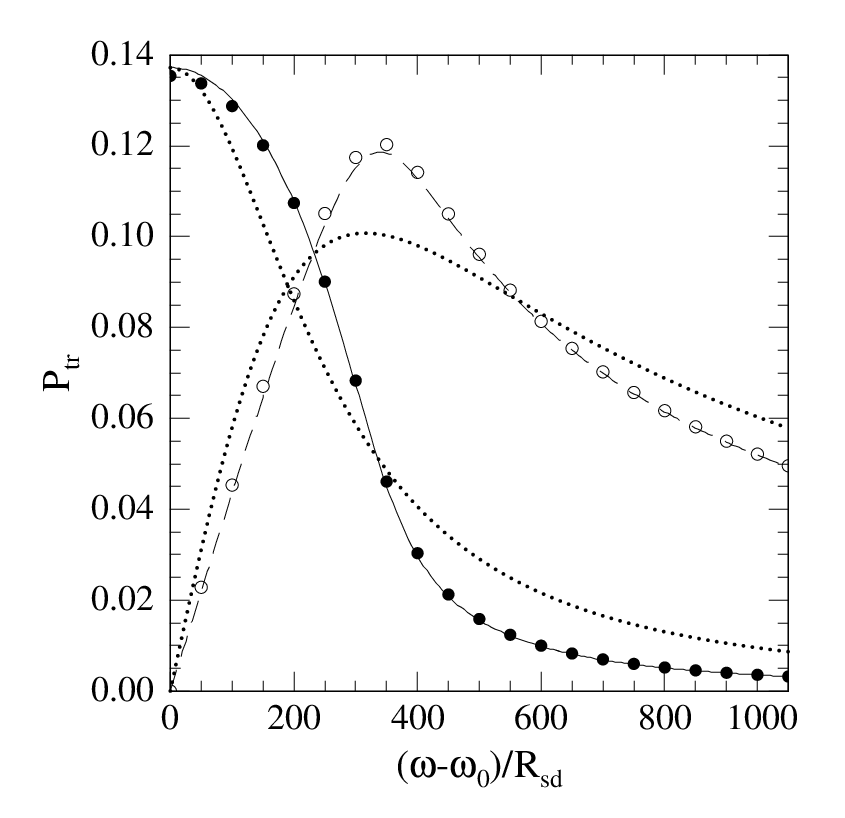
III.3 Comparison of experimental measurements with theory
The results of the simple BE, numerical calculations with the full density matrix equations, and analytical results from the modified BE were compared to a large set of measurements in various parts of the parameter space. One such comparison is shown in Fig. 4. The experimental data compare well to the BE when a variable (from Eq. 11) is used. Note that not only is the measured width greater than that predicted by the simple BE (with constant ) but also, as correctly predicted from the analytical theory, the half-width of the absorption curve differs from the half-width of the dispersion curve. At higher excitation amplitudes, even the modified Bloch analysis begins to deviate from the measured half widths because the polarization begins to drop. The absorbtivity of the vapor also changes as a function of the rf excitation and the pumping rate at the location of the probe beam is not a constant. This can be taken into account by considering the propagation of the pumping light through the polarized vapor. Though the width of the resonance is a good metric for comparing experiment to theory, it is the slope of the dispersive component at resonance that is most important for the magnetometer sensitivity. In Fig. 6 is shown a comparison of the measured slopes (from the same data as Fig. 4) to those predicted by the analytical theory. The agreement is generally satisfactory. In Fig. 7 we show one example of a fit of the measured resonance profile to that predicted from the modified BE. As these data show, in the parameter-space of interest, the modified Bloch analysis provides a good description of the slope and the width of the resonance, as a function of , , , and . Thus we can use these equations to determine the best-achievable sensitivity of the scalar magnetometer.


IV Magnetometer sensitivity
For a given slope of the dispersion curve, unavoidable noise sources in the system determine the fundamental sensitivity of the scalar magnetometer. The calculation of the sensitivity follows closely that for an rf atomic magnetometer, derived in Savukov et al. 2005. For a given polarization noise , the resulting field noise is
| (12) |
There are many sources of technical noise which contribute either directly to the scalar magnetometer noise as in the case of low-frequency magnetic field noise from the current source, or indirectly as in the cases of voltage noise of an amplifier, magnetic field noise at high frequency, vibrations of the optical detection system, and pump laser noise. Technical noise can be removed in principle, so it is important to understand the fundamental limits that determine the best achievable sensitivity.
IV.1 Photon shot noise
In a balanced polarimeter the polarization rotation noise per unit bandwidth due to quantum fluctuations of the number of photons received by photodetectors with quantum efficiency is given by
| (13) |
where is the number of photons per second in the probe beam. The noise has a flat frequency spectrum and is measured in units of rad/Hz1/2. The same level of noise per unit bandwidth will be measured in each phase of a lock-in amplifier calibrated to measure the r.m.s. of an oscillating signal. The optical rotation measured by the lock-in amplifier is given by Eq. (7).
It is convenient to express the photon flux in terms of the pumping rate of the probe beam :
| (14) |
where is the cross-sectional area of the probe beam. If the probe laser is detuned far from resonance, , then one can express photon-atom interactions in terms of the number of absorption lengths on resonance . Using Eq. (12) and magnetometer volume we find the magnetic field noise due to photon shot noise is given by
| (15) |
IV.2 Light-shift noise
The ac Stark shift (light shift) is induced by the probe beam, which is tuned off-resonance from the atomic transition, when it has a non-zero circular polarization. If the probe laser detuning is much larger than the hyperfine splitting, the action of the light on atomic spins is equivalent to the action of a magnetic field parallel to the light propagation direction. This light-shift field is given by (see Eq. (9) of Ref. Savukov et al. 2005),
| (16) |
where is the degree of circular polarization of the probe beam. Light-shift noise can occur as a result of fluctuations of intensity, wavelength, or . If the probe beam is perfectly linearly polarized, fluctuations of the circular polarization are due to quantum fluctuations resulting in an imbalance between the number of left and right circularly polarized photons in the probe beam. The spectral density of the probe beam spin polarization noise is given by . Substituting this value of and excluding by using the pumping rate of the probe beam in the limit we get:
| (17) |
This effective field noise () causes polarization noise by rotating the component into the direction of the primary signal . The amount of polarization noise in induced by the light-shift field is proportional to the spin coherence time . Using simulations of BE with noise terms one can verify that
| (18) |
where a factor appears because only the component of the light-shift field that is co-rotating with the spins contributes to the noise. We get the following contribution of the light shift to the noise of the magnetometer
| (19) |
In most cases of interest here one can assume that .
IV.3 Spin projection noise
The spin-projection noise occurs as a result of quantum fluctuations in the components of atomic angular momentum. We consider the case when the polarization is close to unity and most atoms are in state. Using the fundamental uncertainty relationship with one can show Savukov et al. 2005 that the polarization noise per unit bandwidth is given by
| (20) |
where is the total number of atoms. The spin projection noise depends only weakly on absolute spin polarization; for K atoms with , it increases by for unpolarized atoms. The resulting magnetic field noise in the scalar magnetometer is given by
| (21) |
IV.4 Optimization of fundamental sensitivity
Combining all the noise contributions we obtain the following equation for the magnetometer sensitivity
| (22) |
The first term describes spin projection noise, the second, the light shift of the probe beam, and the third, photon shot noise.
To find the fundamental limit of the sensitivity we assume that can be adjusted separately, for example by increasing the length of the sensing region in the probe direction while keeping the volume constant, or changing the buffer gas pressure. We find that the optimal optical length is equal to . It is always beneficial to reduce and increase , which will result in longer and until . Under optimal probing conditions the fundamental magnetometer sensitivity reduces to
| (23) |
The best sensitivity is obtained by maximizing . For a given and we vary and and calculate and using modified BE with variable given by Eq. (11). We find that for the maximum value of is given by , where . This result is also verified with the full numerical density matrix model. With , the optimal sensitivity of a scalar alkali-metal magnetometer is given by
| (24) |
Hence we find that for a scalar magnetometer the fundamental sensitivity is limited by the rate of spin-exchange collisions even though the resonance linewidth can be much smaller than the spin exchange rate. Numerically for cm2 and we find that fT/Hz1/2 for an active volume of 1 cm3. Using back-action evasion techniques it is possible to make the light shift and photon shot noise contributions negligible, but this only improves the sensitivity to 0.6 fT/Hz1/2 for 1 cm3 volume.
If total noise is limited by photon shot noise or by technical sources of rotation noise, as was the case in our experiment (see Fig. 3), the sensitivity is optimized by maximizing the slope on resonance . Using the same optimization procedure using modified BE and varying and one can obtain . In this case the maximum slope is increased from scaling that one would obtain with a spin-exchange-broadened resonance from Eq. (6). Therefore, light narrowing is useful in reducing the noise in scalar magnetometers limited by photon shot noise or noise, with a maximum sensitivity gain on the order of , which is equal to about 10 for K atoms.
One can also use Eq. (22) to estimate the best sensitivity possible under our actual experimental conditions. In this case the number of absorption length on resonance is not optimal and the spin relaxation of K atoms has additional contribution from collisions with buffer gas and diffusion to the walls. For our parameters corresponding to Fig. 3 (, s-1, s-1, s-1, cm3 and ), including losses in collection of probe light after the cell), we get optimal sensitivity from Eq. (22) of 7 fT/Hz1/2, dominated by photon shot noise. This compares well with the measured photon shot noise level corresponding to 7 fT/Hz1/2 in each channel. The sensitivity could be improved by increasing the resonance optical depth of the vapor.
V Conclusion
In this paper we have systematically analyzed the sensitivity of a scalar alkali-metal magnetometer operating in the regime where the relaxation is dominated by spin-exchange collisions. We demonstrated experimentally magnetic field sensitivity below 10 fT Hz-1/2 with an active volume of 1.5 cm3, significantly improving on previous sensitivities obtained for scalar atomic magnetometers and opening the possibility for further miniaturization of such sensors.
We considered the effects of rf broadening in the presence of SE relaxation and developed a simple analytic model based on Bloch equations with a time that depends on rf excitation. The results of the model have been validated against a complete numerical density matrix calculation and experimental measurements. We showed that the fundamental sensitivity limit for a scalar alkali-metal magnetometer with a 1 cm3 measurement volume is on the order of 0.6-0.9 fT Hz-1/2. In this case a reduction of resonance linewidth by optical pumping of atoms into a stretched state does not lead to an improvement of fundamental sensitivity limit.
It is interesting to compare the scaling of the optimal magnetic field sensitivities in various regimes. It was shown in Kominis et al. 2003 that near zero field in the SERF regime the sensitivity scales as , while for an rf magnetometer operating in a finite field it scales as Savukov et al. 2005. In contrast, here we find that the fundamental sensitivity limited by spin projection noise for a scalar magnetometer in a finite field scales as , i.e. there is no significant reduction of SE broadening for optimal conditions. Since is similar for all alkali metals, one can expect a similar sensitivity for a Cs or Rb magnetometer. On the other hand, if one is limited by the photon shot noise or technical sources of optical rotation noise, which is often the case in practical systems, the magnetometer sensitivity is determined by the slope of the dispersion curve. In this case it is improved in the light-narrowing regime because the slope of the dispersion resonance scales as , instead of for the case of spin-exchanged broadened resonance. We expect similar relationships, with different numerical factors, to hold for atomic clocks operating on the end transitions, since in that case is given by an equation similar to Eq. (11) Y.-Y.Jau et al. 2004. The analytical approach developed in this paper can be easily adapted to other alkali atoms by modifying the coefficients in Eq. (11). This work was supported by an ONR MURI grant.
References
- Knappe et al. (2004) S. Knappe, V. Shah, P. D. D. Schwindt, L. Hollberg, J. Kitching, L.-A. Liew, and J. Moreland, Appl. Phys. Lett. 85, 1460 (2004).
- Groeger et al. (2005) S. Groeger, A. S. Pazgalev, and A. Weis, Appl. Phys. B. 80, 645 (2005).
- Aleksandrov (1995) E. B. Aleksandrov, Opt. and Spectr. 78, 292 (1995).
- Budker et al. (2000) D. Budker, D. F. Kimball, S. M. Rochester, V. V. Yashchuk, and M. Zolotorev, Phys. Rev. A 62, 043403 (2000).
- Happer and Tang (1977) W. Happer and H. Tang, Phys. Rev. Lett. 31, 273 (1977).
- Happer and Tam (1977) W. Happer and A. C. Tam, Phys. Rev. A 16, 1877 (1977).
- Allred et al. (2002) J. C. Allred, R. N. Lyman, T. W. Kornack, and M. V. Romalis, Phys. Rev. Lett. 89, 130801 (2002).
- Appelt et al. (1999) S. Appelt, A. B.-A. Baranga, A. R. Young, and W. Happer, Phys. Rev. A 59, 2078 (1999).
- Y.-Y.Jau et al. (2004) Y.-Y.Jau, A. B. Post, N. N. Kuzma, A. M. Braun, M. V. Romalis, and W. Happer, Phys. Rev. Lett. 92, 110801 (2004).
- Savukov et al. (2005) I. M. Savukov, S. J. Seltzer, M. V. Romalis, and K. L. Sauer, Phys. Rev. Lett. 95, 063004 (2005).
- Kominis et al. (2003) I. K. Kominis, T. W. Kornack, J. C. Allred, and M. V. Romalis, Nature 422, 596 (2003).
- Xia et al. (2006) H. Xia, A. Ben-Amar Baranga, D. Hoffman, and M. V. Romalis, Appl. Phys. Lett. 89, 211104 (2006).
- Lee et al. (2006) S.-K. Lee, K. L. Sauer, S. J. Seltzer, O. Alem, and M. V. Romalis, Appl. Phys. Lett. 89, 214106 (2006).
- Nabighian et al. (2005) M. N. Nabighian, V. J. S. Grauch, R. O. Hansen, T. R. LaFehr, Y. Li, J. W. Peirce, J. D. Phillips, and M. E. Ruder, Geophys. 70, 33ND (2005).
- et al. (2004) A. D. et al., Antiquity 78, 341 (2004).
- Nelson and McDonald (2001) H. H. Nelson and J. R. McDonald, IEEE Trans. Geosci. Remote Sens. 39, 1139 (2001).
- Schwindt et al. (2004) P. D. D. Schwindt, S. Knappe, V. Shah, L. Holberg, and J. Kitching, Appl. Phys. Lett. 85, 6409 (2004).
- Alexandrov et al. (2004) E. B. Alexandrov, M. V. Balabas, A. K. Vershovski, and A. S. Pazgalev, Tech. Phys. 49, 779 (2004).
- Abragam (1961) A. Abragam, Principles of Nuclear Magnetism (Oxford University Press Inc., New York, 1961).
- Bhaskar et al. (1981) N. D. Bhaskar, J. Camparo, W. Happer, and A. Sharma, Phys. Rev. A 23, 3048 (1981).
- Baracchino et al. (1997) L. Baracchino, G. Basso, C. Ciofi, and B. Neri, IEEE Trans. Instrum. Meas. 46, 1256 (1997).
- Savukov and Romalis (2005) I. M. Savukov and M. V. Romalis, Phys. Rev. A 71, 023405 (2005).
- Alexandrov et al. (2002) E. B. Alexandrov, M. V. Balabas, A. Vershovskii, A. I. Okunevich, and N. N. Yakobson, Opt. Spectrosc. 93, 488 (2002).
- Chen et al. (2007) W. C. Chen, T. R. Gentile, T. G. Walker, and E. Babcock, Phys. Rev. A 75, 013416 (2007).
- Appelt et al. (1998) S. Appelt, A. Ben-Amar Baranga, C. J. Erickson, M. V. Romalis, A. R. Young, and W. Happer, Phys. Rev. A 58, 1412 (1998).