Collapse-driven spatiotemporal dynamics of filament formation

From light filaments to Bose Einstein condensates (BEC), from plasma instabilities to hydrodynamical or optical shocks, many nonlinear wave processes lead to self-compression with catastrophic increase in peak intensity, followed by relaxation to a linear state. Universal properties of the compression dynamic were discovered by analyzing the blowup of self-focusing solutions to the nonlinear Schrödinger equation (NSE) FIBICH, described as a self-similar collapse to a smooth and symmetric ground state RYPDAL. Though wave-packets evolve in the three-dimensional (3D) space, uneven initial conditions and compression rates typically lead to symmetry breaking, featured by a transient compression towards a sub-dimensional eigenstate. In light-beam self-focusing, self-similar collapse to the Townes profile (TP), or ground state of the NSE in two spatial dimensions CHIAO, has been recently observed GAETA. As to the subsequent expansion, 3D (space-time) X-waves were shown to capture the apparent stationarity, the pulse-splitting and the conical emission (CE) in the filamentation regime KOLESIK; FACCIO2. Up to date, however, the mechanisms that support the transition from the quasi-2D, self-similar collapse to the 3D relaxation regime remain unrevealed.

A possible approach to this problem requires retaining all highly nonlinear effects relevant to this transition phase in a suitably “dressed” NSE. Here we show that the collapse-driven “morphology” transition from the dominant 2D to the 3D dynamics can be described in the frame of the bare 3D NSE model by the 3D (space-time) instability of the 2D TP eigensate. Up to date, transverse instability was investigated only for the 1D NSE eigenstate KUZNETSOV; RYPDAL2, which however does not support collapse. Our analysis directly applies to light filaments generated by fs pulses in normally dispersive Kerr media, but can be generalized straightforwardly to the collapse in anomalous dispersion, the spatiotemporal (ST) instability of $\chi^{(2)}$ solitons and the collapse of sub-dimensional localized structures in plasmas and BEC. The results capture the key steps of the entire filament evolution from the input Gaussian to the final X waves, and explain the coupling between axial and CE. These were regarded as two independent processes, until recent numerical investigations outlined their simultaneous appearance BRAGHERI. Here the coupling emerges as an intrinsic feature of the instability of the TP, whose signature is a couple of Y-shaped unstable modes. For the first time, a theory is provided that links filamentation, CE, pulse-splitting and supercontinuum generation to the singular behavior at collapse.

Consider the cubic, dimensionless NSE

with $\Delta_{\xi,\eta}=\partial^{2}_{\xi}+\partial^{2}_{\eta}$, for a function $A$ that depends on the spatial coordinates $(\xi,\eta)$ and the temporal coordinate $\tau$. The ground state of the NSE in two spatial dimensions is expressed by $A=a_{0}(\rho)\exp(i\alpha\zeta)$ [$\rho=(\xi^{2}+\eta^{2})^{1/2}$], where $a_{0}(\rho)$ is the TP CHIAO [Fig. 1(a)], and $\alpha\simeq 0.2055$ for the normalization $a_{0}(0)=1$.

Written in the variables $z=(n_{0}/k_{0}n_{2}I)\zeta$, $(x,y)=(n_{0}/k_{0}^{2}n_{2}I)^{1/2}(\xi,\eta)$, $t-k^{\prime}_{0}z=(n_{0}k_{0}^{\prime\prime}/k_{0}n_{2}I)^{1/2}\tau$, $\tilde{A}=I^{1/2}A$, Eq. (1) is a standard model for the propagation of an optical wave packet $E=\tilde{A}(x,y,z,t)\exp(-i\omega_{0}t+ik_{0}z)$ subject to diffraction, normal group velocity dispersion (GVD) ($k_{0}^{\prime\prime}>0$) and self-focusing nonlinearity ($n_{2}>0$) leading to collapse. The ground state describes a monochromatic light beam with $z$-independent transverse amplitude profile. In the above relations, $\omega_{0}$ is the carrier frequency of the wave packet, $I$ is a characteristic intensity, $n_{2}$ the nonlinear refraction index of the medium, and $k(\omega)=n(\omega)\omega/c$ the propagation constant, with $n(\omega)$ the refractive index and $c$ the speed of light in vacuum. Prime signs stand for differentiation with respect to $\omega$, and subscripts 0 for evaluation at $\omega_{0}$.

Following a standard MI analysis, the perturbed TP

with $\sigma\ll 1$, is considered. The ST perturbation will grow exponentially with $\zeta$ if $\kappa_{I}<0$ ($\kappa_{I}\equiv{\rm Im}\kappa$). Opposite frequency shifts $\Omega$ and $-\Omega$ characterize the components $u$ and $v^{\star}$. For simplicity, only cylindrically symmetric perturbations are considered. Introducing (2) into (1), and keeping terms up to the first-order in $\sigma$, one gets the differential eigenvalue problem

where $H=\frac{1}{2}[d^{2}/d\rho^{2}+(1/\rho)d/d\rho+\Omega^{2}]-\alpha+2a_{0}^{2}(\rho)$, with boundary conditions $du(0)/d\rho=dv(0)/d\rho=0$. Given a perturbation frequency $\Omega$, if the problem admits at least one nontrivial solution $(u,v)$ with an eigenvalue $\kappa$ with negative imaginary part, then the TP is unstable under perturbations at that frequency. The problem (3) has to be solved numerically. To simplify the procedure, note first that if $(\kappa,u,v)$ is a solution of (3) at $\Omega$, then $(\kappa^{\star},u^{\star},v^{\star})$, $(-\kappa,v,u)$ and $(-\kappa^{\star},v^{\star},u^{\star})$ are solutions too, whose eigenvalues are all reflections of $\kappa$ about the real and imaginary axes in the complex $\kappa$-plane. Then, if $\kappa$ is complex, only two of these solutions represent unstable perturbations. Following the convention that $\kappa_{R}\geq 0$ ($\kappa_{R}\equiv{\rm Re}\kappa$) and $\kappa_{I}<0$, these two solutions are $(\kappa,u,v)$ and $(-\kappa^{\star},v^{\star},u^{\star})$, that yield the two independent, unstable and physically distinguishable perturbations

since $u$ and $v^{\star}$ are generally different and oppositely frequency shifted in $p_{\kappa}$ and $p_{-\kappa^{\star}}$. Also, any solution of (3) with $\Omega$ is also solution for $-\Omega$. In particular, the unstable solutions $(\kappa,u,v)$ and $(-\kappa^{\star},v^{\star},u^{\star})$ for the perturbation frequency $-\Omega$ are seen from (2) to represent the same but permuted perturbations $p_{-\kappa^{\star}}$ and $p_{\kappa}$. In short, we can restrict the analysis of (3) to $\Omega\geq 0$, and count only eigenvalues with $\kappa_{R}\geq 0$. For each of these with $\kappa_{I}<0$, two independent, unstable perturbations (Collapse-driven spatiotemporal dynamics of filament formation) may grow.

The problem (3) has been solved numerically for each $\Omega\geq 0$ after discretization of the differential operators on a radial ($\rho$) grid of finite size much larger than the Townes range $d\sim 1.5$. Increasing grid points and size allowed to control the accuracy of the results. For $\Omega=0$, no complex eigenvalue is found, as expected from the marginal instability of the TP under pure spatial perturbations RYPDAL2. For each $\Omega>0$, only one, isolated eigenvalue $\kappa$ with $\kappa_{I}<0$ appears, whose real and imaginary parts are shown in Fig. 1(b). The ground state $a_{0}(\rho)\exp(i\alpha\rho)$ is then retrieved to be modulationally unstable under ST perturbations SHEN. The gain $-\kappa_{I}$ is limited to $\Omega\lesssim 1.5$ but without an abrupt cut-off.

For the eigenmodes $u$ and $v$ associated with the complex eigenvalue $\kappa$, some relevant features can be inferred without resorting to numerical calculation. Neglecting terms with $a_{0}^{2}$ in (3) and in $H$ for $\rho\rightarrow\infty$, the decoupled equations $\Delta_{\xi,\eta}u=-[\Omega^{2}-2\alpha-2\kappa]u$ and $\Delta_{\xi,\eta}v=-[\Omega^{2}-2\alpha+2\kappa]v$ are obtained. Their bounded solutions for $\rho\rightarrow\infty$ are $u\propto H_{0}^{(1)}\left[(Q_{u}+i\Gamma_{u})\rho\right]$ and $v\propto H_{0}^{(1)}\left[(Q_{v}+i\Gamma_{v})\rho\right]$, where $H_{0}^{(1)}$ is the Hänkel function of first class and zero order, and the real quantities $Q_{u,v}$ and $\Gamma_{u,v}$ are defined by

with the convention of taking square roots such that $\Gamma_{u,v}\geq 0$. Using that $H^{(1)}_{0}(s)\sim\sqrt{(2/\pi s)}\exp{[i(s-\pi/4)]}$ for large $|s|$, ignoring constant factors and algebraical decay, the expressions $u(\rho)\sim\exp{(-\Gamma_{u}\rho+iQ_{u}\rho)}$ and $v(\rho)\sim\exp{(-\Gamma_{v}\rho+iQ_{v}\rho)}$ are found to describe the dominant behavior of the unstable eigenmodes for large $\rho$. Thus, if their decay rates are small ($\Gamma_{u,v}\ll 1$), $u$ and $v$ are expected to feature radial oscillations of transverse wave numbers $Q_{u,v}$ beyond the TP range.

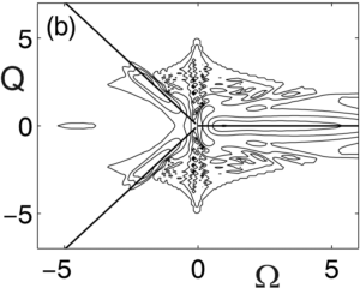
The physical quantities featuring the collapsing dynamics are the growing perturbations $p_{\kappa}$ and $p_{-\kappa^{\star}}$ composed of $u$ and $v$. In particular, the ST spectrum $Q$–$\Omega$ of the unstable perturbations at a certain propagation distance $\zeta$ will be generally expressed by a superposition of the type $\sigma_{\kappa}(\Omega)\hat{p}_{\kappa}(Q,\Omega)+\sigma_{-\kappa^{\star}}(\Omega)\hat{p}_{-\kappa^{\star}}(Q,\Omega)$, where $\hat{p}_{\kappa}(Q,\Omega)$ and $\hat{p}_{-\kappa^{\star}}(Q,\Omega)$ are the spatial Fourier transforms of $p_{\kappa}(\rho,\Omega)$ and $p_{-\kappa^{\star}}(\rho,\Omega)$, and $\sigma_{\kappa}(\Omega)$ and $\sigma_{-\kappa^{\star}}(\Omega)$ are the seeds of each unstable perturbation at each frequency. In experiments, measurement of the ST spectrum $Q$–$\Omega$ (in practice, the angularly-resolved spectrum, displaying angles and wavelengths) of a light filament is a powerful diagnostic in which axial and CE can be visualized at once FACCIO. For the TP, the structure of the $Q$–$\Omega$ spectrum of instability can be inferred from the above asymptotic analysis. The spectrum $\hat{p}_{\kappa}(Q,\Omega)$ is composed of $\hat{u}(Q,\Omega)$ at positive frequency shift $\Omega$ and expectedly peaked at $Q_{u}$, and of $\hat{v}^{\star}(Q,\Omega)$ at negative frequency shift $-\Omega$ and peaked at $Q_{v}$ (if the respective decay rates $\Gamma_{u,v}$ are not large). Plotting $Q_{u}$ and $Q_{v}$ given by (5) versus frequency in their respective ranges, we obtain the black, thick solid curve of Fig. 2(a). This curve is expected to locate the regions in the $Q$–$\Omega$ plane where $\hat{p}_{\kappa}(Q,\Omega)$ takes its highest values. Fig. 2(a) shows also the values of $\Gamma_{u}$ and $\Gamma_{v}$ (black, thin solid curve). Since exponential localization of $v$ is weak ($\Gamma_{v}\ll 1$), the branch $Q_{v}$, fitting approximately the linear relation $Q_{v}\simeq-\sqrt{2}\,\Omega$, is expected to define the locus of maxima of $\hat{v}(Q,\Omega)$, and hence $\hat{p}_{\kappa}(Q,\Omega)$ at down-shifted frequencies to describe an actual off-axis, CE. Instead, localization of $u$ is similar to that of the TP ($\Gamma_{u}\sim 1$) and $Q_{u}$ close to zero, which suggests to associate $\hat{p}_{\kappa}(Q,\Omega)$ at up-shifted frequencies with an axial emission. Similar analysis holds for $\hat{p}_{-\kappa^{\star}}(Q,\Omega)$, CE being now associated with up-shifted frequencies, and axial emission with down-shifted frequencies [see Fig. 2(a), black, dashed curves]. This characterization of the instability spectrum is confirmed by numerical evaluation of $u$ and $v$. Fig. 2(b) shows $\hat{p}_{\kappa}(Q,\Omega)$ with the expected features. Its reflection about $\Omega=0$ yields $\hat{p}_{-\kappa^{\star}}(Q,\Omega)$. The instability of the TP then reveals the link between axial and CE. In this view, the basic ingredients of the ST spectrum of a light filament are not the axial continuum and the X-shaped CE, but two Y-shaped objects, each one coupling off-axis emission to axial emission on opposite frequency bands.

Let us compare these results with those for the ST instability of the plane wave solution $A=\exp(i\zeta)$ to the NSE LIOU. The problem (3) holds for this case if the amplitude $a_{0}$ and the nonlinear wave vector shift $\alpha$ are replaced by unity, and presents the same symmetries. The eigenmodes $u$ and $v$ associated with the most unstable perturbations $p_{\kappa}$ and $p_{-\kappa^{\star}}$ at each frequency $\Omega$ are two plane waves with identical transverse wave numbers $Q_{u}=Q_{v}=\sqrt{\Omega^{2}+2}$. The gain $-\kappa_{I}=1$ is independent of $\Omega$ and hence unbounded. The spectra $\hat{p}_{\kappa}(Q,\Omega)$ and $\hat{p}_{-\kappa^{\star}}(Q,\Omega)$ are then characterized by two identical hyperbolas, depicted in Fig. 2(a) as a single green curve (see Ref. LIOU), and usually referred to as an X-like spectrum. The slope of the X arms is unity, while that of the Y arm is $\sqrt{2}$ ($\sqrt{k_{0}k_{0}^{\prime\prime}}$ against $\sqrt{2k_{0}k_{0}^{\prime\prime}}$ in physical units).

Degeneracy breaking from single X to double Y and gain limitation originate from the transverse localization of the TP. To see this more intuitively, we interpret instability as originated from a Kerr-driven, degenerate four-wave-mixing (FWM) interaction in which two intense, identical pump waves of frequency $\Omega=0$ propagating along the $\zeta$ direction, amplify two weak, non-collinear plane waves, $u$ and $v$, at frequencies $\pm\Omega$. Each pump wave propagates with an axial wave number shift $k_{\rm NL}$ (with respect to a plane wave of frequency $\Omega=0$) due to self-phase modulation (SPM). The axial wave numbers of the weak plane waves are shifted by $\Omega^{2}/2-Q_{u}^{2}/2$ and $\Omega^{2}/2-Q_{v}^{2}/2$ [as obtained from the linearized NSE (1)] due to material dispersion and tilt, and by $k_{{\rm NL},u}$ and $k_{{\rm NL},v}$ due to cross-phase modulation (XPM). Axial phase matching among the interacting waves then reads as

For plane wave pumps, SPM and XPM wave number shifts are $k_{\rm NL}=1$, $k_{{\rm NL},u}=k_{{\rm NL},v}=2k_{\rm NL}=2$ ALFANO. Axial and transverse phase-matching ($Q_{u}^{2}=Q_{v}^{2}$) must be strictly enforced for efficient amplification of $u$ and $v$, which lead to $Q_{u,v}=\sqrt{\Omega^{2}+2}$, i.e., to the X-like spectrum of instability of the plane wave.

Suppose, instead, that the pumps have TPs ($k_{\rm NL}=\alpha$). To account for transverse localization, a) we will assume that plane waves collinear with the pump are preferentially amplified, and b) we take into account that efficient amplification is also possible with small transverse phase-mismatch such that $|Q_{u}-Q_{v}|\lesssim\pi/d$ PENZKOFER. If for instance, the plane wave $u$ at $+\Omega$ is taken as collinear, then $Q_{u}\simeq 0$, and $k_{{\rm NL},u}\simeq 2k_{\rm NL}=2\alpha$. Axial phase matching (6) then requires $Q_{v}\not\simeq 0$, i.e., the plane wave $v$ at $-\Omega$ cannot be collinear. It is then reasonable to take its XPM wave number shift as $k_{{\rm NL},v}\simeq 0$, since the beam does not remain into the localized interaction area FACCIO2. With these assumptions, (6) leads to the linear relation $Q_{v}\simeq-\sqrt{2}\,\Omega$, as for the Y-tail in the instability spectrum of the TP. Limitation of the gain band finds also explanation from the maximum allowed transverse mismatch. If $Q_{u}\simeq 0$, then $Q_{v}\lesssim\pi/d$. Taking $d\simeq 1.5$ for the TP, we obtain $Q_{v}\lesssim 2$, which corresponds roughly to $\Omega\lesssim 1.5$, as obtained above. Obviously, if the collinear plane wave $u$ is taken at $-\Omega$, similar considerations lead to the reflected Y wave.

It follows from our analysis that the onset of downshifted axial emission must be accompanied by upshifted CE, and vice versa, and that these two events may occur independently. Our simulations and experiments support this interpretation. Figure 3(a) shows the ST spectrum of a TP that is not a CW but a pulse. This “perturbed” TP is moreover asymmetric in time by choosing different durations for the leading and trailing parts ($\Delta\tau=0.87$ and $29$, respectively). In Fig. 3(b) the difference between the propagated spectrum under the NSE (1) (distance $\zeta=7.6$) and the input spectrum is shown in order to visualize the newly generated frequencies. A single Y-shaped structure is formed, with a slope of the conical part fitting to $\sqrt{2}$ (thick line).

In the experiments, we used a 15 cm-long fused silica sample as Kerr media. 200-fs-long pulses at 527 nm delivered from a 10 Hz Nd:glass mode-locked and regeneratively amplified system (Twinkle, Light Conversion), were spatially filtered and focused with a 50 cm focal length lens. The pulses then entered into the sample, whose input facet was placed at 52 cm from the lens, and formed a single filament for input energies $E\gtrsim 2\,\mu$J. Angularly resolved spectra of the filament at the output facet and from single laser shots were measured with an imaging spectrometer and a CCD camera, as described in FACCIO. At 2 $\mu$J in fused silica the filament is formed just before the output facet of the sample, the Y-shaped (blue axial, red conical) spectrum of Fig. 3(c) being then observed. At 3 $\mu$J, the filament is formed closer to the input facet. The double Y spectrum of Fig. 3(d) then corresponds to a longer filament path within the sample. The faster growth of one of the two unstable perturbations at the initial stage of filamentation supposes some unbalancing in their seeds. In fact, an expected instability seeding mechanism, as self-phase modulation, generates preferentially axial, blue-shifted frequencies in the presence of plasma and third-order dispersion.

ST instability of the TP also incorporates a mechanism of temporal splitting. If the perturbation $p_{\kappa}$ (e.g.) is seeded coherently at different frequencies, its growth leads to the formation of a pulse, whose spectrum is increasingly peaked at the maximum gain frequencies $\Omega_{M}\simeq 0.365$ for $u$ and $-\Omega_{M}\simeq-0.365$ for $v$. For $u$ and $v$ with respective axial wave number shifts $\kappa_{R}+\alpha$ and $-\kappa_{R}+\alpha$, the inverse group velocity $1/v^{(g)}$ (in the frame moving with the group velocity of a plane pulse at the TP frequency) will be $[d\kappa_{R}/d\Omega|_{\Omega_{M}}]\simeq 0.5$ for $u$, and $[d(-\kappa_{R})/d\Omega|_{-\Omega_{M}}]\simeq 0.5$ for $v$. Being equal, the Y-wave propagates as a whole with a well-defined group velocity. For the $p_{-\kappa^{\star}}$ perturbation, or reflected Y-wave, the group velocity is the opposite, and the group mismatch between the two Y-waves is $1/v^{g}_{p_{\kappa}}-1/v^{(g)}_{p_{-\kappa^{\star}}}\simeq 1$, which in physical variables yields, $\sqrt{k_{0}k_{0}^{\prime\prime}n_{2}I/n_{0}}$, in agreement with the observed dependence in filamentation on pump intensity and material properties FACCIO2.

If the pump is not strictly monochromatic but a long pulse, the Y-waves will leave it at a certain stage, ceasing then to grow. The $p_{\kappa}$ Y-wave behaves then as a linear wave of zero mean frequency and zero axial wave number shifts, since $u$ and $v$, with opposite frequency shifts $\pm\Omega_{M}$, have also opposite axial wave number shifts $\Omega_{M}^{2}/2-Q_{u}^{2}/2\simeq\Omega^{2}_{M}/2$ and $\Omega^{2}_{M}/2-Q_{v}^{2}/2\simeq-\Omega^{2}_{M}/2$. The peculiarity of the linear Y-wave is that the $u$ part experiences the normal GVD $+\Omega^{2}/2$ of the medium, while the $v$ part experiences a net anomalous GVD $-\Omega^{2}/2$ as a result of material and angular dispersion. This makes the $u$ and $v$ parts of $p_{\kappa}$ to continue to depart from the pump at identical group velocity $[d(\Omega^{2}/2)/d\Omega|_{\Omega_{M}}]=[d(-\Omega^{2}/2)/d\Omega|_{-\Omega_{M}}]=\Omega_{M}\simeq 0.365$ (again, the group velocity of the $p_{-\kappa^{\star}}$ Y-wave is the opposite).

Extending our analysis, we may venture an explanation to the fact that two X-waves are commonly observed at later stages of propagation KOLESIK; FACCIO2. Consider, within the FWM approach, the possible effects on the instability spectrum of the strong temporal localization of the pump, as may take place upon (possibly multiple) splitting. For a spatially and temporally localized pump of central frequency $\Omega=0$, axial wave vector shift $k_{\rm NL}$ due to SPM, and propagating at a group velocity $v^{(g)}$ different from that of a plane pulse at $\Omega=0$ (as for an Y-wave), new plane waves $u$ and $v$ at opposite frequencies $\pm\Omega$ are expected to be preferentially amplified if in addition to axial phase matching [Eq. (6)], the velocity of the group formed by $u$ and $v$ matches the velocity of the pump. Equating the inverse beat group velocity $[(\Omega^{2}/2-Q_{u}^{2}/2)-(\Omega^{2}/2-Q_{v}^{2}/2)]/2\Omega$ between $u$ and $v$ to $1/v^{(g)}$, we obtain $Q^{2}_{v}-Q_{u}^{2}=4\Omega/v^{(g)}$. Phase and group matching then yield $Q_{u,v}=\sqrt{\Omega^{2}-(\pm\Omega)/v^{(g)}-2k_{\rm NL}}$ ($+\Omega$ for $u$, $-\Omega$ for $v$), which is the so-called dispersion curve of a frequency-gap X-wave mode PORRAS; FACCIO2. If this process takes place for the two Y-waves with group velocities $1/v^{(g)}=\pm\Omega_{M}$, the two X-waves of Fig. 2(a, red and blue curves) with opposite frequency gaps are generated from the two Y-waves. On nonlinearity relaxation ($k_{\rm NL}\rightarrow 0$) at increasing distances, one branch of each X-wave is seen to pass through the point $Q=\Omega=0$ of the spectrum, as frequently observed KOLESIK; FACCIO2.

In conclusion, Y-waves feature the MI of the TP and constitute the missing links between self-similar spatial self-focusing and ST collapse driven dynamics. Y-waves model the coupling between axial and CE, and allow us to interpret temporal splitting, X-wave formation and final relaxation into linear X-waves. These results provide a unified view of ultrashort pulse filamentation and are relevant to all systems involving ST coupling and nonlinearity such as $\chi^{(2)}$ solitons, BEC, etc.

References

- (1) G. Fibich and G. Papanicolaou, SIAM J. Appl. Math. 60, 183 (1999).
- (2) K. Rypdal and J. J. Rasmussen, Physica Scripta 33, 498 (1986).
- (3) R. Y. Chiao, E. Garmire, and C. H. Townes, Phys. Rev. Lett. 13, 479 (1964).
- (4) K. D. Moll, A. L. Gaeta and G. Fibich, Phys. Rev. Lett. 90, 203902 (2003).
- (5) M. Kolesik, E. M. Wright, and J.V. Moloney, Phys. Rev. Lett. 92, 253901 (2004).
- (6) D. Faccio, et al., Phys. Rev. Lett. 96, 193901 (2006).
- (7) E. A. Kuznetsov, A. M. Rubenchik, and V. E. Zakharov, Phys. Rep. 142, 103 (1986).
- (8) K. Rypdal and J. J. Rasmussen, Physical Scripta 40, 192 (1989).
- (9) F. Bragheri, et al., Phys. Rev. Lett., submitted (2006).
- (10) Y. R. Shen, The principles of nonlinear optics (Wiley- Interscience, New-York, 1984).
- (11) D. Faccio, et al., J. Opt. Soc. Am. B 22, 862 (2005).
- (12) L. W. Liou, X. D. Cao, C. J. McKinstrie and G. P. Agrawal, Phys. Rev. A 46, 4202 (1992).
- (13) R. Alfano and S. Shapiro, Phys. Rev. Lett. 24, 584 (1970).
- (14) A. Penzkofer and H. J. Lehmeier, Opt. Quantum Electron. 25, 815 (1993).
- (15) M. A. Porras and P. Di Trapani, Phys. Rev. E 69, 066606 (2004).