IS THE FERMI FIELD CONTACT AND ISOTROPIC?

Spin magnetic moments of electrons from proper shells of an isolated atom are commonly treated to make two contributions to the hyperfine field $\boldsymbol{B}_{hf}$ on its nucleus [1]. The first is the contact Fermi field produced by $s$-electrons [2], which in the Gauss system of units is equal to

The second is the dipole field created by the distribution of density of spin magnetic moment of electrons from the shells with non-zero orbital moment $l\neq 0$ [1, 3]

In these formulas a nucleus is considered to be placed in the point of origin $r=0$; $\mu_{B}$ is the Bohr magneton; $\boldsymbol{\sigma}$ is the unit vector in the direction of the spin moment of electron; $\Psi\left(\boldsymbol{r}\right)$ - the electron wave function whose subscript in $\left(\ref{Eq1}\right)$, $\left(\ref{Eq2}\right)$ designates only the orbital moment of a shell.

The two fields $\left(\ref{Eq1}\right)$ and $\left(\ref{Eq2}\right)$ are created by two parts of the same distribution of electronic spin moment density. Nevertheless, the contact Fermi field $\left(\ref{Eq1}\right)$ apparently differs from the dipole field $\left(\ref{Eq2}\right)$ in that it is dependent solely on the value of the wave function at $r=0$ whereas the latter is controlled by the distribution of spin density all over around the nucleus. And what is more, the $B_{F}$ value is independent of $\boldsymbol{\sigma}$, while the value of $B_{dip}$ depends on the $\mathbf{\sigma}$ orientation relative to selected directions of the spin density distribution. That is why it seems appropriate to formulate the following questions herein.

(i) Why does not the Fermi field depend on the distribution of spin density all over around the nucleus?

(ii) Why is the multiple in $B_{F}$ equal namely to $8\pi/3$?

(iii) Would the $B_{F}$ value change if the shape of $\Psi_{s}\left(\boldsymbol{r}\right)$ changed whereas the $\Psi_{s}\left(0\right)$ value does not change?

In what follows the answers for these questions are proposed based in part on the results related the field acting on a muon at interstice in solids [4].

In nonrelativistic quantum mechanics just as in classical electrodynamics, magnetic field of any magnetization distribution¹¹ 1 In what follows we will not tell magnetization distribution from the distribution of spin magnetic moment density.

is defined by integral $\left(\ref{Eq2}\right)$. If the point of observation $r=0$ lies inside the distribution and the spin density does not vanish in this point, the under-integral expression diverges. Using standard techniques of calculating the above improper integral (see, for example, [3, 5, 4] ) and assuming that the magnetization changes over the space continuously, one can obtain expression

In the essence, this is simply another form of the standard formula $\boldsymbol{B}=4\pi\boldsymbol{M}\mathbf{+}\boldsymbol{H}$ that defines the magnetic induction inside the magnetization distribution. The first term herein can be called a local because it, as well as the Fermi field, is proportional to the magnetization value at the point of observation, though with another coefficient. The second term in $\left(\ref{Eq4}\right)$ explicitly does not depend on $\boldsymbol{M}\left(0\right)$ and is determined only by the way of changing magnetization over ambient space²² 2 In the classical electrodynamics, it is the latter contribution that, together with allowance for the discontinuity of magnetization on the body surface, determines the demagnetizing field..

Implicitly, however, the magnitude of integral contribution to $\left(\ref{Eq4}\right)$ strongly depends on the $M\left(0\right)$ value. If $M\left(0\right)=0$, as is the case of spin density of electrons from atomic shells with $l\neq 0$ (when this contribution coincides with $\left(\ref{Eq2}\right)$), $M\left(r\right)$ first increases upon moving off a nucleus and then vanishes at $r\rightarrow\infty$. As is easily seen, the regions of increasing and decreasing magnetization with $r$ make contributions of different senses into integral in $\left(\ref{Eq4}\right)$. As a result, the magnitude of hyperfine field is controlled mainly by the distance from a nucleus to the area where spin density is mostly localized, i.e., by the value of parameter $\left\langle r^{-3}\right\rangle$. This designation in [1, 6] was used for the radial part of integral $\left(\ref{Eq2}\right)$, and with the designation for the angular integral part taken also after these authors, one can write the dipole contribution in the form

Unlike is the case when $M\left(0\right)\neq 0$ and magnetization falls monotonically to zero with increasing $r$. Providing the distribution of magnetization is isotropic, $\boldsymbol{M}\left(\boldsymbol{r}\right)=\boldsymbol{M}\left(r\right)$ ($s$-electrons), it vanishes at $r=r_{0}^{\left(1\right)}$ where the first node of the radial $s$-function is located (for $1s$-electrons $r_{0}^{\left(1\right)}\rightarrow\infty$). The integral in $\left(\ref{Eq4}\right)$ over the region $r>r_{0}^{\left(1\right)}$ is equal to zero (see below), and in the range $0<r<r_{0}^{\left(1\right)}$ magnetization only lowers, so that this integral turns out rather large. Besides, because of the spherical symmetry, it does not depend on the form of function $M\left(r\right)$ and always equals $-\frac{4\pi}{3}\boldsymbol{M}\left(0\right)$. It is the sum of two terms in $\left(\ref{Eq4}\right)$ that results in the Fermi field $\left(\ref{Eq1}\right)$.

What would change in the situation described if the part of spin density that does not vanish at $r\mathbf{\rightarrow}0$ is not of spherical symmetry? To answer this question it’s enough to distinguish the two parts of the spin density distribution. The first of them is spherically symmetrical afresh and creates the same field $8\pi\boldsymbol{M}(0)/3$ at the point of observation. The second one has lower symmetry and vanishes in this point, and hence its contribution to the field is described by the formula $\left(\ref{Eq5}\right)$. So the field at the point of observation now is not equal to Fermi field and, which is more, its value depends on $\boldsymbol{M}$ direction.

For instance, in the case of the spin density distribution when the surfaces of constant magnetization have the shape of ellipsoids, a well-known result [5] is obtained from $\left(\ref{Eq4}\right)$

where $\mathcal{N}\left(\mathbf{\sigma}\right)$ is the demagnetizing factor of an ellipsoid. In other words, the magnitude of integral in $\left(\ref{Eq4}\right)$, still remaining proportional to $M\left(0\right)$, turns out dependent also on the direction of spin moment, which is designated as previously by symbol $\mathbf{\sigma}$. For the spherically symmetrical distribution of magnetization this dependence disappears, $\mathcal{N}\left(\mathbf{\sigma}\right)\equiv 1/3$ so that $4\pi\left(1-\mathcal{N}\right)=8\pi/3$ and one comes again to the Fermi field $\left(\ref{Eq1}\right)$.

Let us discuss now how local expressions $\left(\ref{Eq1}\right)$ and $\left(\ref{Eq6}\right)$ arise from the integral in $\left(\ref{Eq4}\right).$ The matter is that a homogeneously magnetized layer that lies between two similar ellipsoidlike surfaces (in particular, spherical layer) does not produce the field inside [5]. Representing the whole magnetization distribution in the form of an ”onion” consisting of such closely adjoined layers, we can take off any external layers without changing field in the center ³³ 3 It is just the reason for the part of spin density of $s$-electron from the region $r>r_{0}^{\left(1\right)}$ to not contribute to hyperfine field.. As a result, the field in the center turns out coinciding with the field of an infinitely small homogeneously magnetized ellipsoid, and the same conclusion follows from the common simple method of calculating Fermi field [3] as well.

However, it does not mean that the Fermi field is produced solely by the infinitesimal central part of the spin density. It means only that for some spin density distributions of high symmetry (in particular spherical, cubic and ellipsoid-like symmetry) the sum of contributions to $\boldsymbol{B}_{hf}$, produced by the outer parts of the distribution, becomes equal to zero. This is not true for the spin density distributions of lower symmetry, and to make matters worse, in this case one can not find unambiguously the part of the spin density that does not vanish in the point of observation, i.e. the part that should create the “contact” field. If, in addition to this, one takes into account the $\boldsymbol{B}_{hf}$ anisotropy, which is absent only in a spherically symmetrical case $\left(\ref{Eq1}\right)$, to infer on the ”locality” is hardly pertinent.

Could, however, one expect that in an atom there is a part of spin density that would lower monotonically and anisotropically upon moving off the nucleus? It is impossible of course in an isolated atom, but it may be the case in a crystal of low-symmetry. Apparently, it is how, for example, the density of itinerant electrons in crystals with the lattice symmetry lower than cubic should behave. The simplest argument in favor of this quite evident statement can be obtained in the approximation of almost free electrons. Consider an electronic state $\left|\boldsymbol{k}\right\rangle=\exp\left(i\boldsymbol{kr}\right)$ in the rhombic $\Gamma_{0}$-type lattice. Let the perturbation potential has the form

If the $V$ value is quite small comparing to the change of kinetic energy of an electron $\varepsilon\left(\boldsymbol{k}\right)=\frac{\hslash^{2}k^{2}}{2m}$, in the lowest order of the perturbation theory, six states $\left|k_{x}+\alpha\frac{2\pi}{a},k_{y},k_{z}\right\rangle$, $\left|k_{x},k_{y}+\alpha\frac{2\pi}{b},k_{z}\right\rangle$, $\left|k_{x},k_{y},k_{z}+\alpha\frac{2\pi}{c}\right\rangle$, $\ \alpha=\pm 1$ are mixed to each state $\left|\boldsymbol{k}\right\rangle$ with one and the same matrix element $V$. Hence, the charge $\rho\left(\boldsymbol{r}\right)$ and spin magnetic moment $M\left(\boldsymbol{r}\right)$ density of an electron acquire an inhomogeneous addendum proportional to

Hence, the distribution of spin density around the point of origin (the nucleus of one of the atoms constituent the lattice) is already anisotropic. In the vicinity of a nucleus, isolines of spin density turn out to have the form of ellipsoids elongated the stronger, the greater is the difference in lattice parameters $a,b$ and $c$.

Similar anisotropy should arise in the opposite limiting case as well, i.e. in the tight binding approximation, if to allow for the fact that the wave functions of neighbors overlap the stronger, the closer they are located. To make it evident, a study of the simplest case of a two-atom molecule is sufficient. Let us treat an ionized hydrogen molecule $H_{2}^{+}$ in which atomic nuclei have the coordinates $\boldsymbol{r}_{1}$and $\boldsymbol{r}_{2}$, with the vector $\boldsymbol{R}=\boldsymbol{r}_{2}-\boldsymbol{r}_{1}$ being parallel to the $z$ axis. The ground-state wave function is chosen in the form

Here, $\rho=R/a$, $a=a_{0}/Z$ is the radius of the $1s$ orbit, which at $R\longrightarrow\infty$ is equal to the Bohr radius $a_{0}$ and decreases when the atoms come closer [7]. This effect is taken into account via introduction of an effective nucleus charge $Z$ whose value is conditioned at each $R$ by the minimal average energy of the state $\left(\ref{Eq9}\right)$.

The spin magnetization distribution in this state is the sum of two contributions:

The magnetization distribution $\boldsymbol{M}_{1}\left(\boldsymbol{r}\right)$ creates at every nucleus the magnetic field induction:

This result can easily be obtained after simple reasoning similar to the above with account for the fact that a homogeneously magnetized sphere creates around the same field as a point dipole placed in the center of the sphere and having magnetic moment equal to that of the sphere.

The formula $\left(\ref{Eq11}\right)$ looks like the standard expression for calculation of the field at an atomic nucleus in a crystal, which includes the Fermi contribution and the dipole fields created by the neighboring magnetic atoms. However, in this case, the homogeneous and equal to $\mathbf{\sigma}\exp\left(-2\rho\right)/Q^{2}$ part of the spin density distribution, which is concentrated inside the sphere with a radius $R$ and the center located at the neighboring site, contributes solely to the Fermi field. The dipole field is given rise to only by a heterogeneous part of this distribution so that the magnetic moment entering into $\boldsymbol{B}_{dip}$ $\left(\ref{Eq11}\right)$ is equal

As a result, with decreasing $R$, the anisotropic contribution $B_{dip}$ reaches its maximum and vanishes at $R\rightarrow 0$, rather then increases proportionally to $1/R^{3}$.

The second contribution to the magnetization $\boldsymbol{M}_{2}\left(\boldsymbol{r}\right)$ arises because of the interference of the atomic states in $\left(\ref{Eq9}\right)$. The surfaces $M_{2}\left(\boldsymbol{r}\right)=const$ are the ellipsoids of revolution, with the eccentricity tending to zero at $\left|\boldsymbol{r}-\boldsymbol{r}_{1}\right|+\left|\boldsymbol{r}-\boldsymbol{r}_{2}\right|\longrightarrow R$. Again, with the considerations similar to the above-employed, it is easy to show that the contribution of $\boldsymbol{M}_{2}$ into the magnetic field induction has the same value and direction at the nuclei and at every point of the segment that connects them. Just as the Fermi field, this contribution is proportional to the magnitude $\boldsymbol{M}_{2}\left(\boldsymbol{r}\right)$, which is constant at every point of the segment and equal to $-2\mu_{B}\mathbf{\sigma}\exp\left(-\rho\right)/Q^{2}$. Therefore, the field induction related to $\boldsymbol{M}_{2}$ is determined by the formula similar to $\left(\ref{Eq6}\right)$:

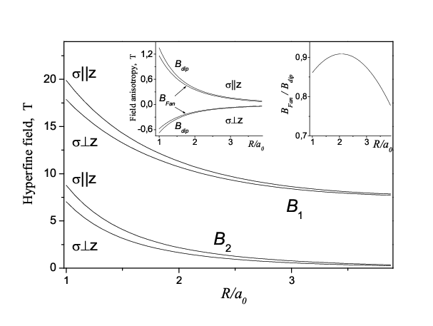
The dependences of $B_{1}$ and $B_{2}$ on $R/a_{0}$ at $\boldsymbol{\sigma}\mathbf{\parallel}z$ and $\boldsymbol{\sigma}\mathbf{\perp}z$ are shown in the Figure 1 and corresponding dependences of the anisotropic contributions to $B_{1}$ and $B_{2}$, i.e., $B_{dip}\mathbf{\left(\boldsymbol{\sigma}\right)}$ and $B_{Fan}\mathbf{\left(\boldsymbol{\sigma}\right)=}B_{\mathbf{2}}\mathbf{\left(\boldsymbol{\sigma}\right)-}\left[B_{\mathbf{2}}\mathbf{\left(\boldsymbol{\sigma}\mathbf{\parallel}\overset{\char 94\relax}{z}\ \right)+2}B_{\mathbf{2}}\mathbf{\left(\boldsymbol{\sigma}\mathbf{\perp}\overset{\char 94\relax}{z}\right)}\right]/3$, are displayed in the first insert. The total anisotropy value makes up about 10% $\left|\boldsymbol{B}_{1}+\boldsymbol{B}_{2}\right|$, and the Fermi-field anisotropy turns out only slightly lower than the dipole field anisotropy, as is seen from the second insert in the same figure.

Thus, in the $H_{2}^{+}$ molecule, with decreasing spacing, not only the hyperfine field at the nuclei as such increases (chemical shift) but its anisotropy as well. In this case, about half the anisotropy contribution is ascribed to the anisotropic part of the Fermi field related to hybridization of the atomic orbitals. The same effect should evidently arise also in crystals in which the distances from a magnetic ion to its closest neighbors in different directions strongly vary, which leads to various overlapping of their outer $s$-shells.

In general, the value of local contribution to the induction $\left(\ref{Eq4}\right)$ is controlled by the form of dependence $div\left(\boldsymbol{M}\right)$ on coordinates. If the spin part of the wave function does not depend on $\boldsymbol{r}$, i.e. $\boldsymbol{M}\left(\boldsymbol{r}\right)$ is directed parallel to $z$-axe in any point, $div\left(\boldsymbol{M}\right)$ has the form

The first term in this formula having been integrated on $\boldsymbol{r}$ in $\left(\ref{Eq4}\right)$ always gives $-\frac{4\pi}{3}M\left(0\right)$. The result of the integration of the second term in common case is the functional of $M\left(\boldsymbol{r}\right)$. In particular, if $M\left(\boldsymbol{r}\right)=\mathcal{M}\left(r\right)\Phi\left(\theta,\varphi\right)$, as is the case for atomic states with $l\neq 0$, the value of this functional depends on $\left\langle r^{-3}\right\rangle$ just as in $\left(\ref{Eq5}\right)$. For the result of this integration to be, alike the Fermi field $\left(\ref{Eq6}\right)$, proportional solely to $M\left(0\right)$, the $M\left(\boldsymbol{r}\right)$ dependence should have the special form

where $\mathcal{M}$ and $\Phi$ are any sufficiently smooth functions. Taking into account that in this case

we obtain replacing $\left(\ref{Eq14}\right)$ and $\left(\ref{Eq16}\right)$ into $\left(\ref{Eq4}\right)$:

The atomic $s$-state is a trivial (the angular dependence is absent) particular case of spin density distribution $\left(\ref{Eq15}\right)$. The other examples of distributions of this type are ellipsoid-like distribution or a distribution with cubic symmetry.

In order that the spin density distribution for an isolated atom turns out a function of the type $\left(\ref{Eq15}\right)$, its ground state should be mixed to by the states of the continuous spectrum. Such mixing up actually arises when an atom is located in an electrical field, in particular, the crystalline electrical field. However, calculation of the corresponding contribution to the Fermi field is a serious mathematical problem, which requires special treatment.

Returning to the questions posed at the beginning of the paper, we now can formulate the following conclusions.

(i) The contact contribution to the induction at internal point of any magnetization distribution virtually results from the summing up of the fields created by all elements of this distribution.

(ii) The value of the proportionality coefficient between the induction and magnetic moment density at a point of observation is controlled by the symmetry of the magnetization distribution. This coefficient is isotropic and equal to $8\pi/3$ only for distributions with a spherical or cubical symmetry.

(iii) In molecules and crystals of a lower symmetry owing to the hybridization of the states of neighboring atoms, the symmetry of the $s$-electron density distribution around the nucleus decreases. This results not only in the proportionality coefficient between the induction and magnetic-moment density at the point of observation changes, but starts depend on the moment direction.

It should be underlined also, that the main result of this paper reduces to the substantiation of a very simple statement: individualization of the Fermi field from the total hyperfine field becomes empty of meaning for low-symmetry crystals and molecules. The calculation of the field created by a spin density distribution of low symmetry should be performed by the formula $\left(\ref{Eq4}\right)$ or some equivalent to it. The standard presentation of hyperfine field as the sum of the Fermi $\left(\ref{Eq1}\right)$, dipole and Lorentz fields and demagnetizing field of the specimen results in masking the role of the spin density inhomogeniouties, which may be the source of some faults.

Allowance for this circumstance may be quite important when analyzing the results of the hyperfine field measurements. The case in hand may be both the fields acting on a probe particle (neutron, muon and others) in the interstices [4], and the field on an atomic nucleus in a crystal or molecule. In all these cases, with a proper account for the contribution of collective electrons and/or distortions of the atomic $s$-shells, additional anisotropic contributions to the Fermi field can emerge. In particular, one could not exclude that the high (up to $3\div 4\quad T$) anisotropy of the hyperfine field at the nuclei of iron atoms that constitute the dumb-bells in the compounds $R_{2}Fe_{17}$ [8, 9, 10] is related to this effect rather then to unquenching of orbital moments.

Acknowledgments

I am grateful to Prof. V.V. Dyakin for useful discussions.

This work has been partly supported by Russian Academy of Sciences, grant 02-02-16440 and Ural Division of RAS, project No 5.

References

- [1] Bleaney B 1967 Hyperfine interactions Acad. Press, (NY-L) p.15
- [2] Ferm E 1930 Zs. f. Phys. 60 320
- [3] White R M 1983 Quantum theory of magnetism. (Springer-Verlag. Berlin, NY) ch. 2
- [4] Rosenfeld E V and Irkhin Yu P 1999 Izv. Acad. Nauk Russia Ser. Phys., 63 1375; Rosenfeld E V and Irkhin Yu P 1998 Phys. Metal. Metalloved. 86 37
- [5] Tamm I E 1989 Fundamentals of theory of electricity (Nauka,. Moscow) ch.5
- [6] Watson R E and Freeman A J 1967 Hiperfine interactions (Acad. Press, NY-L) p.62
- [7] Fermi E 1984 Notes on quantum mechanics (University of Chicago Press) p. 290
- [8] van der Kraan A M, Gubbens P G M and Bushow K H J 1975 Phys. stat. sol. (a) 31 495
- [9] Gubbens P C M and Bushow K H J 1973 Appl. Phys. 44 3739
- [10] Averbuch-Pouchot M T, Chevalier R, Deportes J, Kebe B and Lemaire R 1987 JMMM 68 190