Frozen light in photonic crystals with degenerate band edge

Alex Figotin Ilya Vitebskiy

Abstract

Consider a plane monochromatic wave incident on a semi-infinite periodic structure. What happens if the normal component of the transmitted wave group velocity vanishes? At first sight, zero normal component of the transmitted wave group velocity simply implies total reflection of the incident wave. But we demonstrate that total reflection is not the only possible outcome. Instead, the transmitted wave can appear in the form of a frozen mode with very large diverging amplitude and either zero, or purely tangential energy flux. The field amplitude in the transmitted wave can exceed that of the incident wave by several orders of magnitude. There are two qualitatively different kinds of frozen mode regime. The first one is associated with a stationary inflection point of electromagnetic dispersion relation. This phenomenon has been analyzed in our previous publications. Now, our focus is on the frozen mode regime related to a degenerate photonic band edge. An advantage of this new phenomenon is that it can occur in much simpler periodic structures. This spectacular effect is extremely sensitive to the frequency and direction of propagation of the incident plane wave. These features can be very attractive in a variety practical applications, such as higher harmonic generation and wave mixing, light amplification and lasing, highly efficient superprizms, etc.

1 Introduction

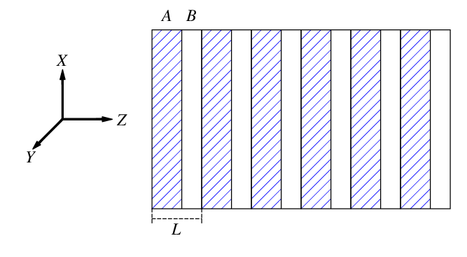
Wave propagation in spatially periodic media, such as photonic crystals, can be qualitatively different from any uniform substance. The differences are particularly pronounced when the wavelength is comparable to the primitive translation $L$ of the periodic structure [1, 2, 3, 4, 5, 6, 7]. The effects of strong spatial dispersion culminate when the group velocity $u=\partial\omega/\partial k$ of a traveling Bloch wave vanishes. One reason for this is that vanishing group velocity always implies a dramatic increase in density of modes at the respective frequency. In addition, vanishing group velocity also implies certain qualitative changes in the eigenmode structure, which can be accompanied by some spectacular effects in electromagnetic wave propagation. A particular example of the kind is the frozen mode regime associated with a dramatic enhancement of the wave transmitted to the periodic medium [8, 9, 10, 11, 12, 13]. There are at least two qualitatively different modifications of the frozen mode regime, each related to a specific singularity of the electromagnetic dispersion relation. Both effects can be explained using the simple example of a plane electromagnetic wave normally incident on a lossless semi-infinite periodic structure, as shown in Fig. 1.

Refer to caption — Figure 1: Plane wave normally incident on a semi-infinite photonic crystal. The subscripts $I$ , $R$ , and $T$ refer to the incident, reflected and transmitted waves, respectively. In all cases, the amplitude of the incident wave is unity.

The frozen mode regime of the first kind is associated with a stationary inflection point on the $k-\omega$ diagram shown in Fig. 2(b). In the vicinity of stationary inflection point, the relation between the frequency $\omega$ and the Bloch wave number $k$ can be approximated as

\omega-\omega_{0}\propto\left(k-k_{0}\right)^{3}.

(1)

A monochromatic plane wave of frequency close to $\omega_{0}$ incident on semi-infinite photonic crystal is converted into the frozen mode with infinitesimal group velocity and dramatically enhanced amplitude, as illustrated in Fig. 3. The saturation value of the frozen mode amplitude diverges as the frequency approaches its critical value $\omega_{0}$ . Remarkably, the photonic crystal reflectivity at $\omega=\omega_{0}$ can be very low, implying that the incident radiation is almost totally converted into the frozen mode with zero group velocity, diverging amplitude, and finite energy flux close to that of the incident wave [9, 10, 11].

A qualitatively different kind of frozen mode regime is expected in the vicinity of a degenerate photonic band edge shown in Fig. 2(c). This case is the main focus of our investigation. At frequencies just below $\omega_{d}$ , the dispersion relation can be approximated as

\omega_{d}-\omega\propto\left(k-k_{d}\right)^{4},\text{ at }\omega\lessapprox\omega_{d}.

(2)

Contrary to the case of stationary inflection point (1), in the vicinity of a degenerate band edge the photonic crystal becomes totally reflective. But at the same time, the steady-state field inside the periodic medium (at $z>0$ ) develops a very large amplitude, diverging as the frequency approaches its critical value $\omega_{d}$ . Such a behavior is illustrated in Fig. 4. The frozen mode profile below and above the degenerate band edge frequency $\omega_{d}$ is different. It has a large saturation value at frequencies located inside the transmission band (at $\omega\leq\omega_{d}$ ), as seen in Fig. 4(a) and (b). This saturation value diverges as $\omega\rightarrow\omega_{d}-0$ . By contrast, at frequencies inside the band gap (at $\omega>\omega_{d}$ ), the field amplitude initially increases dramatically with the distance $z$ from the surface, but then vanishes as the distance $z$ further increases, as seen in Fig. 4(d – f).

Figs. 3 and 4 describe the frozen mode profile in hypothetical lossless semi-infinite periodic media. In the case of a photonic crystal with finite thickness, the frozen mode profile remains unchanged in the leftmost portion of the periodic structure in Fig. 1. In the opposite, rightmost part of the photonic crystal, the frozen mode amplitude vanishes, as illustrated in Fig. 5. Additional factors limiting the frozen mode amplitude include structural imperfections of the periodic array, absorption, nonlinearity, deviation of the incident radiation from plane monochromatic wave, etc. Still, with all these limitations in place, the frozen mode regime can be very strong.

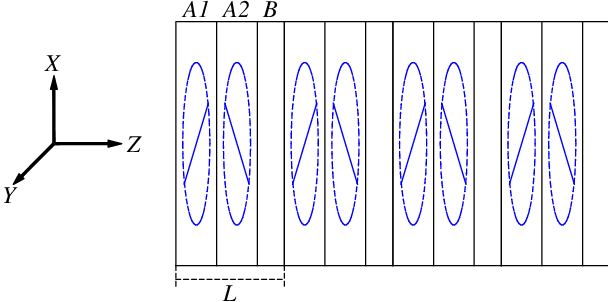
Not every periodic structure can support the frozen mode regime at normal incidence. Generally, the physical conditions for the frozen mode regime are the same as the conditions for the existence of the respective stationary point (1) or (2) of the dispersion relation. In either case, a unit cell of the periodic layered structure must contain at least three layers, of which two must display a misaligned in-plane anisotropy, as shown in Fig. 6. The difference, though, is that a stationary inflection point (1) also required the presence of magnetic layers with strong nonreciprocal circular birefringence [8, 9]. No magnetic layers are needed for a degenerate band edge (2), which constitutes a major practical advantage of the respective frozen mode regime. In photonic crystals with three dimensional periodicity, the presence of anisotropic constitutive component may not be necessary. A detailed comparative analysis of the above two modifications of the frozen mode regime at normal incidence is carried out in the next section. The emphasis is on the physical conditions under which these phenomena can occur.

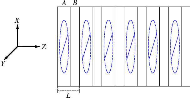
In Section 3, we turn to the case of oblique wave propagation. The frozen mode regime at oblique incidence can occur when the normal component of the transmitted wave group velocity vanishes, while its tangential component remains finite. In such a case, the transmitted wave is an abnormal grazing mode with a dramatically enhanced amplitude and nearly tangential energy flux. A significant advantage of the oblique modification of the frozen mode regime is that it can occur in much simpler periodic structures, compared to those supporting the frozen mode regime at normal incidence. Examples are shown in Figs. 7 and 8. The presence of anisotropic layers is still required.

Yet another interesting modification of the frozen mode regime are abnormal subsurface wave. Such waves can exist at band gap frequencies close to a degenerate photonic band edge. Regular surface waves usually decay exponentially with the distance from the surface in either direction. By contrast, abnormal subsurface waves are extremely asymmetric. They do decay rapidly outside the photonic crystal. But inside the periodic medium, their amplitude sharply increases, and reaches its maximum at a certain distance from the surface. Only after that the field amplitude begins a slow decay, as the distance from the surface further increases. The profile of a subsurface wave is similar to that of the frozen mode above the degenerate band edge in Fig. 4(d – f). This phenomenon is briefly discussed in section 4.

In Section 5 we discuss the physical requirements to the spatially periodic arrays capable of supporting the frozen mode regime, both at normal and oblique incidence. We also present a detailed description of the periodic layered structures used in our numerical simulations.

Finally, in Section 6 we summarize the results and discuss some physical limitations of the frozen mode regime.

2 The physical nature of the frozen mode regime

The essence of the frozen mode regime can be understood from the simple example of a plane monochromatic wave normally incident on a semi-infinite periodic layered structure, as shown in Fig. 1. An important requirement, though, is that some of the layers display a misaligned in-plane anisotropy as shown in the example in Fig. 6. Below we present a comparative analysis of two different kinds of frozen mode regime. Although throughout this section we only consider the case of normal incidence, in the next section we will show that most of the results and expressions remain virtually unchanged in a more general case of the frozen mode regime at oblique propagation. One difference, though, is that at oblique incidence, the frozen mode regime can occur in much simpler structures. This can have a big advantage in practical terms.

To start with, let us introduce some basic notations and definitions. Let $\Psi_{I}$ , $\Psi_{R}$ , and $\Psi_{T}$ be the incident, reflected and transmitted waves, respectively. Assume for now that all three monochromatic waves propagate along the $z$ axis normal to the surface of semi-infinite periodic layered structure in Fig. 1. Electromagnetic field both inside (at $z>0$ ) and outside (at $z<0$ ) the periodic stack is independent of the $x$ and $y$ coordinates. The transverse field components can be represented as a column-vector

\Psi\left(z\right)=\left[\begin{array}[]{c}E_{x}\left(z\right)\\ E_{y}\left(z\right)\\ H_{x}\left(z\right)\\ H_{y}\left(z\right)\end{array}\right],

(3)

where $\vec{E}\left(z\right)$ and $\vec{H}\left(z\right)$ are time-harmonic electric and magnetic fields. All four transverse field components in (3) are continuous functions of $z$ , which leads to the following standard boundary condition at $z=0$

\Psi_{T}\left(0\right)=\Psi_{I}\left(0\right)+\Psi_{R}\left(0\right).

(4)

Assume also that anisotropic layers of the periodic array have an in-plane anisotropy (69), in which case the fields $\vec{E}\left(z\right)$ and $\vec{H}\left(z\right)$ are normal to the direction of propagation

\vec{E}\left(z\right)\perp z,\vec{H}\left(z\right)\perp z,

(5)

and the column vector (3) includes all nonzero field components. Note that the polarizations of the incident, reflected and transmitted waves can be different, because some of the layers of the periodic array display an in-plane anisotropy, as shown in the example in Fig. 6. The presence of anisotropic layers is essential for the possibility of frozen mode regime.

In periodic layered media, the electromagnetic eigenmodes $\Psi_{k}\left(z\right)$ are usually chosen in the Bloch form

\Psi_{k}\left(z+L\right)=e^{ikL}\Psi_{k}\left(z\right),

(6)

where the Bloch wavenumber $k$ is defined up to a multiple of $2\pi/L$ . The correspondence between $\omega$ and $k$ is referred to as the Bloch dispersion relation. Real $k$ correspond to propagating (traveling) Bloch modes. Propagating modes belong to different spectral branches $\omega\left(k\right)$ separated by frequency gaps. The speed of a traveling wave in a periodic medium is determined by the group velocity [4]

u=d\omega/dk.

(7)

Normally, each spectral branch $\omega\left(k\right)$ develops stationary points $\omega_{s}=\omega\left(k_{s}\right)$ where the group velocity (7) of the corresponding propagating mode vanishes

d\omega/dk=0\text{, at }\omega=\omega_{s}=\omega\left(k_{s}\right).\text{ }

(8)

Examples of different stationary points are shown in Fig. 2, where each of the frequencies $\omega_{g}$ , $\omega_{0}$ and $\omega_{d}$ is associated with zero group velocity of the respective traveling wave. Stationary points (7) play essential role in the formation of frozen mode regime.

By contrast, evanescent Bloch modes are characterized by complex wavenumbers $k=k^{\prime}+ik^{\prime\prime}$ . Evanescent modes decay exponentially with the distance $z$ from the boundary of semi-infinite periodic structure. Therefore, under normal circumstances, evanescent contribution to the transmitted wave $\Psi_{T}\left(z\right)$ can be significant only in close proximity of the surface. The situation can change dramatically when the frequency $\omega$ approaches one of the stationary point values $\omega_{s}$ . At first sight, stationary points (8) relate only to propagating Bloch modes. But in fact, in the vicinity of every stationary point frequency $\omega_{s}$ , the imaginary part $k^{\prime\prime}$ of the Bloch wavenumber of at least one of the evanescent modes also vanishes. As a consequence, the respective evanescent mode decays very slowly, and its role may extend far beyond the photonic crystal boundary. In addition, in the special cases of interest, the electromagnetic field distribution $\Psi\left(z\right)$ in the coexisting evanescent and propagating eigenmodes becomes very similar, as $\omega$ approaches $\omega_{s}$ . This can result in spectacular resonance effects, such as the frozen mode regime. What exactly happens in the vicinity of a particular stationary point (8) essentially depends on its character and appears to be very different in each of the three cases presented in Fig. 2.

In the next subsection we present a simple qualitative picture of the frozen mode regime based solely on energy conservation consideration. This will allow us to highlight the difference between the cases of stationary inflection point (1) and degenerate band edge (2). Then, we discuss the physical nature of the frozen mode regime.

2.1 Energy density and energy flux at frozen mode regime

Let $S_{I}$ , $S_{R}$ and $S_{T}$ be the energy flux in the incident, reflected and transmitted waves in Fig. 1. The transmission and reflection coefficients of a lossless semi-infinite medium are defined as

\tau=\frac{S_{T}}{S_{I}},\ \rho=-\frac{S_{R}}{S_{I}},

(9)

where

S_{I}+S_{R}=S_{T},~\rho=1-\tau.

With certain reservations, the energy flux $S_{T}$ of the transmitted travelling wave can be expressed as

S_{T}=W_{T}u,

(10)

where $u$ is the group velocity, which is also the energy velocity, and $W_{T}$ is the energy density

W_{T}\propto\left|\Psi_{T}\right|^{2}.

Evanescent modes do not contribute to the normal energy flux $S_{T}$ in the case of a lossless semi-infinite periodic structure. Besides, evanescent contribution to the transmitted wave becomes negligible at a certain distance $z$ from the surface. The simple expression (10) may not apply when the transmitted wave involves two or more propagating Bloch modes, but we will not deal with such a situation here.

Vanishing group velocity $u$ in (10) implies that the transmitted wave energy flux $S_{T}$ also vanishes, along with the respective transmission coefficient $\tau$ in (9). The only exception could be if the energy density $W_{T}$ of the transmitted wave increases dramatically in the vicinity of the stationary point frequency. In other words, if $W_{T}$ in (10) grows fast enough, as $\omega$ approaches $\omega_{s}$ , the product $W_{T}u$ in (10) can remain finite even at $\omega=\omega_{s}$ . In such a case, a significant fraction of the incident radiation can be converted into the slow mode inside the semi-infinite periodic array. The effect of a dramatic growth of the transmitted wave amplitude in the vicinity of a stationary point (8) will be referred to as the frozen mode regime. The possibility of such an effect is directly related to the character of a particular stationary point. From this point of view, let us consider three different situation presented in Fig. 2.

2.1.1 Regular band edge

We start with the simplest case of a regular photonic band edge (RBE) in Fig. 2(a). It can be found in any periodic array, including any periodic layered structure. Just below the band edge frequency $\omega_{g}$ , the dispersion relation can be approximated by a quadratic parabola

\omega_{g}-\omega\propto\left(k-k_{g}\right)^{2},\text{ at }\omega\lessapprox\omega_{g}.

(11)

This yields the following frequency dependence of the propagating mode group velocity $u$ inside the transmission band

u=\frac{d\omega}{dk}\propto\left(k_{g}-k\right)\propto\left(\omega_{g}-\omega\right)^{1/2},\text{ at }\omega\lessapprox\omega_{g}.

(12)

Due to the boundary condition (4), the amplitude of the transmitted propagating Bloch mode remains finite and comparable to that of the incident wave. Therefore, the energy flux (10) associated with the transmitted slow mode vanishes, as $\omega$ approaches $\omega_{g}$

S_{T}=W_{T}u\propto\left\{\begin{array}[]{c}\left(\omega_{g}-\omega\right)^{1/2},\text{ at }\omega\lessapprox\omega_{g}\\ 0,\text{ at }\omega\geq\omega_{g}\end{array}\right..

(13)

Formula (13) expresses the well-known fact that in the vicinity of a regular photonic band edge, a lossless semi-infinite photonic crystal becomes totally reflective.

2.1.2 Stationary inflection point

A completely different situation occurs in the vicinity of a stationary inflection point in Fig. 2(b). At normal propagation, such a point can be found in periodic layered structures involving anisotropic and magnetic layers [8, 9], as well as in some photonic crystals with 2- and 3-dimensional periodicity. In the vicinity of a stationary inflection point $\omega_{0}$ , the dispersion relation can be approximated by a cubic parabola (1). The propagating mode group velocity $u$ vanishes as $\omega$ approaches $\omega_{0}$ from either direction

u=\frac{d\omega}{dk}\propto\left(k-k_{0}\right)^{2}\propto\left(\omega-\omega_{0}\right)^{2/3}.

(14)

But remarkably, the amplitude of the transmitted propagating mode increases so that the respective energy density $W_{T}$ diverges as $\omega\rightarrow\omega_{0}$

W_{T}\propto\left(\omega-\omega_{0}\right)^{-2/3}.

(15)

The expression (14) together with (15) yield that the energy flux of the transmitted slow mode remains finite even at $\omega=\omega_{0}$

S_{T}=W_{T}u\sim S_{I},\text{ at }\omega\approx\omega_{0}.

(16)

The latter implies that the incident light is converted to the frozen mode with infinitesimal group velocity (14) and diverging amplitude (15). This result was first reported in [9]. A consistent analytical description of the asymptotic behavior of the transmitted field amplitude in the vicinity of a stationary inflection point was carried out in [13].

2.1.3 Degenerate band edge

Let us turn to the case of a degenerate band edge in Fig. 2(c). At normal propagation, such a point can be found in dispersion relation of periodic layered structures with misaligned anisotropic layers. An example is shown in Fig. 6. Just below the degenerate band edge frequency $\omega_{d}$ , the dispersion relation $\omega\left(k\right)$ can be approximated by a biquadratic parabola (2). This yields the following frequency dependence of the propagating mode group velocity inside the transmission band

u=\frac{d\omega}{dk}\propto\left(k_{d}-k\right)^{3}\propto\left(\omega_{d}-\omega\right)^{3/4},\text{ at }\omega\lessapprox\omega_{d}.

(17)

Analysis shows that the amplitude of the transmitted slow mode in this case diverges, as the frequency approaches the band edge value

W_{T}\propto\left|\omega_{d}-\omega\right|^{-1/2},\text{ }\ \ \text{at }\omega\lessapprox\omega_{DBE},

(18)

which constitutes the frozen mode regime. But the energy density (18) does not grow fast enough to offset the vanishing group velocity (17). The expressions (17) and (18) together with (10) yield for the energy flux

S_{T}=W_{T}u\propto\left\{\begin{array}[]{c}\left(\omega_{d}-\omega\right)^{1/4},\text{ at }\omega\lessapprox\omega_{d}\\ 0,\text{ at }\omega\geq\omega_{d}\end{array}\right.,

(19)

implying that, in spite of the diverging energy density (18), the energy flux of the transmitted slow wave vanishes, as $\omega$ approaches $\omega_{d}$ .

The situation at a degenerate band edge (2) can be viewed as intermediate between the frozen mode regime at a stationary inflection point (1), and the vicinity of a regular band edge (11). Indeed, on the one hand, the incident wave at $\omega=\omega_{d}$ is totally reflected back to space, as is the case at a regular band edge. On the other hand, the transmitted field amplitude inside the periodic medium diverges as $\omega\rightarrow\omega_{d}$ , which is similar to what occurs at a stationary inflection point.

The above consideration does not explain the nature of the frozen mode regime, nor does it address the problem of the Bloch composition of the frozen mode. These questions are the subject of the next subsection.

2.2 Bloch composition of frozen mode

In a periodic layered structure, at any given frequency $\omega$ , there are four electromagnetic eigenmodes with different polarizations and wavenumbers. But in the setting of Fig. 1, where the semi-infinite periodic array occupies the half-space $z\geq 0$ , the transmitted wave is a superposition of only two of the four Bloch eigenmodes. Indeed, neither the propagating modes with negative group velocity, nor evanescent modes exponentially growing with the distance $z$ from the surface, contribute to $\Psi_{T}\left(z\right)$ in this case. Generally, one can distinguish three different possibilities.

1.

Both Bloch components of the transmitted wave $\Psi_{T}$ are propagating modes

$\Psi_{T}\left(z\right)=\Psi_{pr1}\left(z\right)+\Psi_{pr2}\left(z\right),\ \;z\geq 0.$ (20)

$\Psi_{pr1}\left(z\right)$ and $\Psi_{pr2}\left(z\right)$ are two propagating Bloch modes with different real wavenumbers $k_{1}$ and $k_{2}$ and different group velocities $u_{1}>0$ and $u_{2}>0$ . This constitutes the phenomenon of double refraction, provided that $u_{1}$ and $u_{2}$ are different. The other two Bloch components of the same frequency have negative group velocities and cannot contribute to the transmitted wave $\Psi_{T}$ .
2.

Both Bloch components of $\Psi_{T}$ are evanescent

$\Psi_{T}\left(z\right)=\Psi_{ev1}\left(z\right)+\Psi_{ev2}\left(z\right),\ \;z\geq 0.$ (21)

The respective two values of $k$ are complex with positive imaginary parts $k^{\prime\prime}>0$ . This is the case when the frequency $\omega$ falls into photonic band gap at $\omega>\omega_{g}$ in Fig. 2(a) or at $\omega>\omega_{d}$ in Fig. 2(c). The fact that $k^{\prime\prime}>0$ implies that the wave amplitude decays with the distance $z$ from the surface. In the case (21), the incident wave is totally reflected back to space by the semi-infinite periodic structure.
3.

One of the Bloch components of the transmitted wave $\Psi_{T}$ is a propagating mode with $u>0$ , while the other is an evanescent mode with $k^{\prime\prime}>0$

$\Psi_{T}\left(z\right)=\Psi_{pr}\left(z\right)+\Psi_{ev}\left(z\right),\ \;z\geq 0.$ (22)

For example, this is the case at $\omega\sim\omega_{0}$ in Fig. 2(b), as well as at $\omega<\omega_{g}$ in Fig. 2(a) and at $\omega<\omega_{d}$ in Fig. 2(c). As the distance $z$ from the surface increases, the evanescent contribution $\Psi_{ev}$ in (22) decays as $\exp\left(-zk^{\prime\prime}\right)$ , and the resulting transmitted wave $\Psi_{T}\left(z\right)$ turns into a single propagating Bloch mode $\Psi_{pr}$ .

Propagating modes with $u>0$ and evanescent modes with $k^{\prime\prime}>0$ are referred to as forward waves. Only forward modes contribute to the transmitted wave $\Psi_{T}\left(z\right)$ in the case of a periodic semi-infinite stack. The propagating modes with $u<0$ and evanescent modes with $k^{\prime\prime}<0$ are referred to as backward waves. The backward waves never contribute to the transmitted wave $\Psi_{T}$ inside the periodic semi-infinite stack in Fig. 1. This statement is based on the following two assumptions:

-

The transmitted wave $\Psi_{T}$ and the reflected wave $\Psi_{R}$ are originated from the plane wave $\Psi_{I}$ incident on the semi-infinite photonic slab from the left, as shown in Fig. 1.
-

The layered array in Fig. 1 occupies the entire half-space and is perfectly periodic at $z>0$ .

If either of the above conditions is violated, the electromagnetic field inside the periodic stack can be a superposition of four Bloch eigenmodes with either sign of the group velocity $u$ of propagating contributions, or either sign of $k^{\prime\prime}$ of evanescent contributions. This would be the case if the periodic layered array in Fig. 1 had some kind of structural defects or a finite thickness. At the end of this section we briefly discuss how it would affect the frozen mode regime.

Note also that the assumption that the transmitted wave $\Psi_{T}\left(z\right)$ is a superposition of propagating and/or evanescent Bloch eigenmodes may not apply if the frequency $\omega$ exactly coincides with one of the stationary point frequencies (8). For example, at frequency $\omega_{0}$ of stationary inflection point (1), there are no evanescent solutions to the Maxwell equations (54), and the transmitted wave $\Psi_{T}\left(z\right)$ is a (non-Bloch) Floquet eigenmode linearly growing with $z$ [9, 10]. Similar situation occurs at frequency $\omega_{d}$ of degenerate band edge (2). The term ”non-Bloch” means that the respective field distribution does not comply with the relation (6). At the same time, at any general frequency, including the vicinity of any stationary point (8), the transmitted wave $\Psi_{T}\left(z\right)$ is a superposition of two Bloch eigenmodes, each of which is either propagating, or evanescent.

In all three cases (20 – 22), the contribution of a particular Bloch eigenmode to the transmitted wave $\Psi_{T}$ depends on the polarization $\Psi_{I}$ of the incident wave. One can always choose some special incident wave polarization, such that only one of the two forward Bloch modes is excited and the transmitted wave $\Psi_{T}$ is a single Bloch eigenmode. In the next subsection we will see that there is no frozen mode regime in the case of a single mode excitation. This fact relates to the very nature of the frozen mode regime.

Knowing the Bloch composition of the transmitted wave we can give a semi-qualitative description of what happens when the frequency $\omega$ of the incident wave approaches one of the stationary points (8) in Fig. 2. More consistent analysis based on the Maxwell equations is outlined in Section 4.

2.2.1 Regular photonic band edge

We start with the simplest case of a regular photonic band edge. There are two different possibilities in this case, but none of them is associated with the frozen mode regime. The first one relates to the trivial case where none of the layers of the periodic structure displays an in-plane anisotropy or gyrotropy. As the result, all eigenmodes are doubly degenerate with respect to polarization. A detailed description of this case can be found in the extensive literature on optics of stratified media [2, 3]. Slightly different scenario occurs if some of the layers are anisotropic or gyrotropic and, as a result, the polarization degeneracy is lifted. Just below the band edge frequency $\omega_{g}$ in Fig. 2(a), the transmitted field $\Psi_{T}\left(z\right)$ is a superposition (22) of one propagating and one evanescent Bloch modes. Due to the boundary condition (4), the amplitude of the transmitted wave at $z=0$ is comparable to that of the incident wave. In the case of a generic polarization of the incident light, the amplitudes of the propagating and evanescent Bloch components at $z=0$ are also comparable to each other and to the amplitude of the incident light

\left|\Psi_{pr}\left(0\right)\right|\sim\left|\Psi_{ev}\left(0\right)\right|\sim\left|\Psi_{I}\right|,\text{ at }\ \omega\leq\omega_{g}.

(23)

As the distance $z$ from the surface increases, the evanescent component $\Psi_{ev}\left(z\right)$ decays rapidly, while the amplitude of the propagating component remains constant. Eventually, at a certain distance from the slab surface, the transmitted wave $\Psi_{T}\left(z\right)$ becomes very close to the propagating mode

\Psi_{T}\left(z\right)\approx\Psi_{pr}\left(z\right),\text{ at }z\gg L,\ \omega\leq\omega_{g}.

(24)

The evanescent component $\Psi_{ev}$ of the transmitted wave does not display any singularity at the band edge frequency $\omega_{g}$ . The propagating mode $\Psi_{pr}$ does develop a singularity associated with vanishing group velocity at $\omega\rightarrow\omega_{g}-0$ , but its amplitude remains finite and comparable to that of the incident wave. At $\omega>\omega_{g}$ , this propagating mode turns into another evanescent mode in (21). The bottom line is that none of the Bloch components of the transmitted wave develops a large amplitude in the vicinity of a regular photonic band edge. There is no frozen mode regime in this trivial case.

2.2.2 Stationary inflection point

A completely different situation develops in the vicinity of a stationary inflection point (1) of the dispersion relation. At $\omega\approx\omega_{0}$ , the transmitted wave $\Psi_{T}$ is a superposition (22) of one propagating and one evanescent Bloch component. In contrast to the case of a regular photonic band edge, in the vicinity of $\omega_{0}$ both Bloch contributions to $\Psi_{T}$ develop strong singularity. Specifically, as the frequency $\omega$ approaches $\omega_{0}$ , both contributions grow dramatically, while remaining nearly equal and opposite in sign at the slab boundary [9]

\Psi_{pr}\left(0\right)\approx-\Psi_{ev}\left(0\right)\propto\left|\omega-\omega_{0}\right|^{-1/3},\ \ \text{as }\omega\rightarrow\omega_{0}.

(25)

Due to the destructive interference (25), the resulting field

\Psi_{T}\left(0\right)=\Psi_{pr}\left(0\right)+\Psi_{ev}\left(0\right)

at the surface at $z=0$ is small enough to satisfy the boundary condition (4). As the distance $z$ from the slab boundary increases, the destructive interference becomes less effective – in part because the evanescent contribution decays exponentially

\Psi_{ev}\left(z\right)\approx\Psi_{ev}\left(0\right)\exp\left(-zk^{\prime\prime}\right),

(26)

while the amplitude of the propagating contribution remains constant and very large. Eventually, the transmitted wave $\Psi_{T}\left(z\right)$ reaches its large saturation value corresponding to its propagating component $\Psi_{pr}$ , as seen in Fig. 9(a).

Note that the imaginary part $k^{\prime\prime}$ of the evanescent mode wavenumber in (26) also vanishes in the vicinity of stationary inflection point

k^{\prime\prime}\propto\left|\omega-\omega_{0}\right|^{1/3}\text{, as }\omega\rightarrow\omega_{0},

(27)

reducing the rate of decay of the evanescent contribution (26). As a consequence, the resulting amplitude $\Psi_{T}\left(z\right)$ of the transmitted wave reaches its large saturation value $\Psi_{pr}$ in (25) only at a certain distance $Z$ from the surface.

Z\propto 1/k^{\prime\prime}\propto\left|\omega-\omega_{0}\right|^{-1/3}.

(28)

This characteristic distance diverges as the frequency approaches its critical value $\omega_{0}$ .

If the frequency of the incident wave is exactly equal to the frozen mode frequency $\omega_{0}$ , the transmitted wave $\Psi_{T}\left(z\right)$ does not reduce to the sum (22) of propagating and evanescent contributions, because at $\omega=\omega_{0}$ , there is no evanescent solutions to the Maxwell equations (54). Instead, $\Psi_{T}\left(z\right)$ corresponds to a non-Bloch Floquet eigenmode diverging linearly with $z$ [9].

\Psi_{T}\left(z\right)-\Psi_{T}\left(0\right)\propto z\Psi_{0},\;\ \text{at}\;\omega=\omega_{0}.

(29)

Such a solution is shown in Fig. 3(c).

2.2.3 Degenerate band edge

While the situation with a regular photonic band edge (11) appears trivial, the case of a degenerate band edge (2) proves to be quite different. Just below the degenerate band edge frequency $\omega_{d}$ (inside the transmission band), the transmitted field is a superposition (22) of one propagating and one evanescent components. Above $\omega_{d}$ (inside the band gap), the transmitted wave is a combination (21) of two evanescent components. In this respect, a regular and a degenerate band edges are similar to each other. A crucial difference, though, is that in the vicinity of a degenerate band edge, both Bloch contributions to the transmitted wave diverge as $\omega$ approaches $\omega_{d}$ , both above and below the band edge frequency. This constitutes the frozen mode regime.

Let us start with the transmission band. As the frequency $\omega$ approaches $\omega_{d}-0$ , both Bloch contributions in (22) grow sharply, while remaining nearly equal and opposite in sign at the surface

\Psi_{pr}\left(0\right)\approx-\Psi_{ev}\left(0\right)\propto\left|\omega_{d}-\omega\right|^{-1/4},\ \ \text{as }\omega\rightarrow\omega_{d}-0.

(30)

This asymptotic formula was obtained in [13] using the perturbation theory for the $4\times 4$ transfer matrix (67). The destructive interference (30) ensures that the boundary condition (4) can be satisfied, while both Bloch contributions to $\Psi_{T}\left(z\right)$ diverge. As the distance $z$ from the slab boundary increases, the evanescent component $\Psi_{ev}\left(z\right)$ dies out

\Psi_{ev}\left(z\right)\approx\Psi_{ev}\left(0\right)\exp\left(-zk^{\prime\prime}\right)

(31)

while the propagating component $\Psi_{pr}\left(z\right)$ remains constant and very large. Eventually, as the distance $z$ further increases, the transmitted wave $\Psi_{T}\left(z\right)$ reaches its large saturation value corresponding to its propagating component $\Psi_{pr}\left(z\right)$ , as illustrated in Fig. 10. Note that the imaginary part $k^{\prime\prime}$ of the evanescent mode wavenumber also vanishes in the vicinity of degenerate band edge

k^{\prime\prime}\propto\left|\omega-\omega_{d}\right|^{1/4}\text{, as }\omega\rightarrow\omega_{d},

(32)

reducing the rate of decay of the evanescent contribution (31). As a consequence, the resulting amplitude $\Psi_{T}\left(z\right)$ of the transmitted wave reaches its large saturation value $\Psi_{pr}$ only at a certain distance $Z$ from the surface

Z\propto 1/k^{\prime\prime}\propto\left|\omega-\omega_{d}\right|^{-1/4}.

(33)

This characteristic distance increases as the frequency approaches its critical value $\omega_{d}$ , as illustrated in Fig. 4(a) and (b).

If the frequency $\omega$ of the incident wave is exactly equal to $\omega_{d}$ , the transmitted wave $\Psi_{T}\left(z\right)$ does not reduce to the sum of two Bloch contributions. Instead, it corresponds to a non-Bloch Floquet eigenmode linearly diverging with $z$

\Psi_{T}\left(z\right)-\Psi_{T}\left(0\right)\propto z\Psi_{d},\;\ \text{at}\;\omega=\omega_{d}.

(34)

This situation is shown in Fig. 4(c).

The above behavior appears to be very similar to that of the frozen mode regime at a stationary inflection point, shown in Figs. 3 and 9. Yet, there is a crucial difference between the frozen mode regime at a stationary inflection point and at a degenerate band edge. According to (19), in the immediate proximity of a degenerate band edge, the Pointing vector $S_{T}$ of the transmitted wave is infinitesimal, in spite of the diverging wave amplitude (30). In other words, although the energy density $W_{T}\propto\left|\Psi_{T}\right|^{2}$ of the frozen mode diverges as $\omega\rightarrow\omega_{d}-0$ , it does not grow fast enough to offset the vanishing group velocity (17). As a consequence, the photonic crystal becomes totally reflective at $\omega=\omega_{d}$ . Of course, the total reflectivity persists at $\omega>\omega_{d}$ , where there is no propagating modes at all. By contrast, in the case (29) of a stationary inflection point, the respective Pointing vector $S_{T}$ is finite and can be even close to that of the incident wave, implying low reflectivity and nearly total conversion of the incident wave energy into the frozen mode.

The character of frozen mode regime is different when we approach the degenerate band edge frequency from the band gap. In such a case, the transmitted field $\Psi_{T}\left(z\right)$ is a superposition (21) of two evanescent components. As the frequency $\omega$ approaches $\omega_{d}$ , both evanescent contributions grow sharply, while remaining nearly equal and opposite in sign at the photonic crystal boundary

\Psi_{ev1}\left(0\right)\approx-\Psi_{ev2}\left(0\right)\propto\left|\omega_{d}-\omega\right|^{-1/4},\ \ \text{as }\omega\rightarrow\omega_{d}+0.

(35)

This asymptotic formula also was derived using the perturbation theory for the $4\times 4$ transfer matrix (67). Again, the destructive interference (35) ensures that the boundary condition (4) is satisfied, while both evanescent contributions to $\Psi_{T}\left(z\right)$ diverge in accordance with (35). As the distance $z$ from the slab boundary increases, the destructive interference of these two evanescent components is lifted and the resulting field amplitude increases sharply, as seen in Fig. 11(a). But eventually, as the distance $z$ further increases, the transmitted wave $\Psi_{T}\left(z\right)$ completely decays, because both Bloch contributions to $\Psi_{T}\left(z\right)$ are evanescent. The latter constitutes the major difference between the frozen mode regime above and below the DBE frequency $\omega_{d}$ . The rate of the amplitude decay, as well as the position of the maximum of the transmitted wave amplitude in Figs. 4(d – f) and 11(a) , are characterized by the distance $Z$ in (33).

2.2.4 Physical reason for the growing wave amplitude

If the frequency $\omega$ is close, but not equal, to that of a stationary point (8) of the dispersion relation, the wave $\Psi_{T}\left(z\right)$ transmitted to the semi-infinite periodic layered medium is a superposition of two forward Bloch modes $\Psi_{1}\left(z\right)$ and $\Psi_{2}\left(z\right)$

\Psi_{T}\left(z\right)=\Psi_{1}\left(z\right)+\Psi_{2}\left(z\right).

(36)

The two Bloch modes in (36) can be a propagating and an evanescent, as in (22), or they can be both evanescent, as in (21). In the vicinity of frozen mode regime, as the frequency approaches its critical value ( $\omega_{0}$ or $\omega_{d}$ ), the two Bloch eigenmodes contributing to $\Psi_{T}\left(z\right)$ become nearly indistinguishable from each other

\Psi_{1}\left(z\right)\approx\alpha\Psi_{2}\left(z\right),\ \ \text{as }\omega\rightarrow\omega_{s},

(37)

where $\alpha$ is a scalar, and $\omega_{s}$ is the frozen mode frequency ( $\omega_{0}$ or $\omega_{d}$ ). The asymptotic relation (37) reflects a basic property of the transfer matrix (61) of periodic layered structures at frequency of either a stationary inflection point, or a degenerate band edge. A rigorous analysis based on the perturbation theory and leading to (37) is carried out in [13]. For more on this see the Section 4.

Let us show under what circumstances the property (37) can lead to the frozen mode regime. The sum (36) of two nearly parallel column vectors $\Psi_{1}$ and $\Psi_{2}$ must match the boundary conditions (4) with the incident and reflected waves. If the incident wave polarization is general, then the nearly parallel Bloch components $\Psi_{1}$ and $\Psi_{2}$ must be very large and nearly equal and opposite

\Psi_{1}\left(0\right)\approx-\Psi_{2}\left(0\right),\ \ \left|\Psi_{1}\left(0\right)\right|\approx\left|\Psi_{2}\left(0\right)\right|\gg\left|\Psi_{I}\right|,

(38)

in order to satisfy the boundary conditions (4). Indeed, since the incident field polarization is general, we have no reason to expect that the column vector $\Psi\left(0\right)$ at the surface is nearly parallel to $\Psi_{1}\left(0\right)$ and $\Psi_{2}\left(0\right)$ . But on the other hand, the boundary conditions say that

\Psi\left(0\right)=\Psi_{1}\left(0\right)+\Psi_{2}\left(0\right)

(39)

Obviously, the only situation where the sum (39) of two nearly parallel vectors can be not nearly parallel to either of them is the one described in (38).

There is one exception, though. As we already stated in (37), in the vicinity of the frozen mode frequency, the two Bloch components $\Psi_{1}$ and $\Psi_{2}$ of the transmitted wave are nearly parallel to each other. For this reason, if the polarization of the incident wave $\Psi_{I}$ is such that $\Psi\left(0\right)$ in (39) is nearly parallel to one of the Bloch eigenmodes $\Psi_{1}\left(0\right)$ or $\Psi_{2}\left(0\right)$ , it is also nearly parallel to the other one. So, all three column vectors $\Psi_{1}\left(0\right)$ , $\Psi_{2}\left(0\right)$ , and $\Psi\left(0\right)$ are now parallel to each other. In this, and only this case, the amplitude of the transmitted wave $\Psi_{T}\left(z\right)$ will be comparable to that of the incident wave. There is no frozen mode regime for the respective vanishingly small range of the incident wave polarization. A particular case of the above situation is a regime of a single mode excitation, where only one of the two Bloch components $\Psi_{1}$ or $\Psi_{2}$ in (36) contributes to the transmitted wave.

Finally, let us reiterate that in the limiting cases of $\omega=\omega_{0}$ or $\omega=\omega_{d}$ , the transmitted wave $\Psi_{T}\left(z\right)$ corresponds to the non-Bloch Floquet eigenmode (29) or (34), respectively. Either of them linearly diverges with $z$ . Again, the only exception is when the incident wave has the unique polarization, at which the transmitted wave $\Psi_{T}\left(z\right)$ is a propagating Bloch eigenmode with zero group velocity and a limited amplitude, comparable to that of the incident wave. Incident wave with any other polarization will generate the frozen mode inside the periodic medium.

2.3 Frozen mode regime in bounded photonic crystals

The above consideration was based on the assumption that the transmitted wave is a superposition of only forward waves, which include propagating modes with $u>0$ and/or evanescent modes with $k^{\prime\prime}>0$ . This assumption, reflected in (20), (21), and (22), does not apply to bounded photonic crystals, where the periodic medium does not occupy the entire half-space $z>0$ . If the periodic layered array in Fig. 1 has a finite thickness, the electromagnetic field inside the periodic stack is a superposition of all four Bloch eigenmodes with either sign of the group velocity $u$ of propagating contributions, and/or either sign of $k^{\prime\prime}$ of evanescent contributions. How does a finite thickness affect the frozen mode regime? In Fig. 5, we depicted the frozen mode profile in periodic stacks composed of different number $N$ of identical unit cells $L$ in Fig. 6. The total thickness of the respective photonic slab is equal to $NL$ . In all cases, the incident wave frequency $\omega$ coincides with that of the degenerate band edge $\omega_{d}$ in (11). The presence of the second (right-hand) boundary of the periodic array gives rise to the backward wave contribution to $\Psi_{T}\left(z\right)$ . Comparison of Fig. 5(a – c) to the semi-infinite case in Fig. 5(d) shows that the backward wave contribution to the formation of the frozen mode profile becomes significant only at a certain distance from the surface of incidence at $z=0$ . Specifically, the backward wave contribution eliminates the frozen mode in the right-hand portion of the finite photonic slab, while having no impact in its left-hand portion at $0<z\ll NL$ . Similar situation occurs at the frozen mode regime associated with stationary inflection point (1). Importantly, the frozen mode profile near the surface of incidence is not affected by the finite dimensions of the photonic crystal.

In addition to the modification of the frozen mode profile, the bounded photonic crystals of relatively small dimensions can display strong Fabry-Perot cavity resonances, also known as transmission band edge resonances. The respective resonance frequencies are located strictly inside the transmission band (see, for example, [14], and references therein) and do not interfere with the frozen mode regime. Cavity resonances are distinct from the frozen mode regime and go outside the scope of our investigation.

3 Frozen mode regime at oblique propagation – abnormal grazing modes

A phenomenon similar to the frozen mode regime can also occur at oblique wave propagation, where the incident, reflected and transmitted waves are all propagate at an angle to the $z$ axis, as shown in Fig. 12. Consider the situation where the normal component $u_{z}$ of the group velocity of the transmitted propagating wave vanishes, while the tangential component $\vec{u}_{\perp}$ remains finite.

u_{z}=\frac{\partial\omega}{\partial k_{z}}=0,\ \ \vec{u}_{\perp}=\frac{\partial\omega}{\partial\vec{k}_{\perp}}\neq 0\text{, at }\omega=\omega_{s}=\omega\left(\vec{k}_{s}\right).

(40)

This is exactly what happens in the vicinity of the well-known phenomenon of total internal reflection [6]. Similar effect occurs in any photonic crystal at frequency corresponding to the transmission band edge for a particular direction of incidence. Remarkably, the total reflection of the incident wave is not the only possible outcome. Another alternative is that the transmitted wave forms an abnormal grazing mode with dramatically enhanced amplitude and tangential energy flux. The profile of such a grazing mode, i.e., the field dependence on the distance $z$ from the surface, appears to be very similar to that of the frozen mode at normal incidence shown in Figs. 3 and 4. The only difference is that the tangential component of the transmitted wave group velocity now remains finite and can even be comparable to the speed of light in vacuum.

A significant advantage of the oblique version of the frozen mode regime is that it can occur in much simpler periodic structures, compared to those supporting the frozen mode regime at normal incidence. Examples of periodic layered arrays supporting only the oblique version of the frozen mode regime are shown in Figs. 7 and 8. These structures are too simple to support any kind of frozen mode regime at normal incidence – they have only two different layers in a unit cell $L$ , of which only one layer is anisotropic. But at oblique incidence, these relatively simple periodic arrays can support the frozen mode regime. The presence of at least one anisotropic layer in a unit cell $L$ is still required. The physical requirements to periodic structures capable of supporting both normal and oblique versions of the frozen mode regime are discussed in Section 5.

3.1 Axial dispersion relation – basic definitions

Consider a plane monochromatic wave obliquely incident on a periodic semi-infinite stack, as shown in Fig. 12. Due to the boundary conditions (4), the incident, reflected, and transmitted waves should be assigned the same pair of tangential components $k_{x},k_{y}$ of the respective wave vectors

\left(\vec{k}_{I}\right)_{x}=\left(\vec{k}_{R}\right)_{x}=\left(\vec{k}_{T}\right)_{x},\ \ \left(\vec{k}_{I}\right)_{y}=\left(\vec{k}_{R}\right)_{y}=\left(\vec{k}_{T}\right)_{y},

(41)

while the axial (normal) components $k_{z}$ are all different. For the incident and reflected waves we have simply

\left(\vec{k}_{I}\right)_{z}=-\left(\vec{k}_{R}\right)_{z}=\sqrt{\omega^{2}c^{2}-k_{x}^{2}-k_{y}^{2}}.

(42)

Let us turn to the transmitted wave. The transmitted wave is usually a composition of two Bloch eigenmodes with the same $\vec{k}_{\perp}=\left(k_{x},k_{y}\right)$ from (41), but different $k_{z}$ and different polarizations. For given $\vec{k}_{\perp}$ and $\omega$ , the value of $k_{z}$ is obtained by solving the time-harmonic Maxwell equations (52) in the periodic medium. The so-obtained correspondence between the wavenumber $k_{z}$ and the frequency $\omega$ at fixed $\vec{k}_{\perp}$ is referred to as the axial or normal dispersion relation. Real $k_{z}$ correspond to propagating (traveling) Bloch modes, while complex $k_{z}$ correspond to evanescent modes, decaying with the distance $z$ from the surface. Unlike $k_{x}$ and $k_{y}$ , the Bloch wavenumber $k_{z}$ is defined up to a multiple of $2\pi/L$ .

Similarly to the case of normal propagation, the expression (40) defines stationary points of the axial dispersion relation. The definition (40) is a generalization of (8) to the case of oblique propagation. Different kinds of axial stationary points are defined as follows.

-

A regular band edge of axial dispersion relation

$\frac{\partial\omega}{\partial k_{z}}=0,\ \frac{\partial^{2}\omega}{\partial k_{z}^{2}}\neq 0.$ (43)
-

A stationary inflection point of axial dispersion relation

$\frac{\partial\omega}{\partial k_{z}}=0,\ \frac{\partial^{2}\omega}{\partial k_{z}^{2}}=0,\ \frac{\partial^{3}\omega}{\partial k_{z}^{3}}\neq 0.$ (44)

A degenerate band edge of axial dispersion relation

\frac{\partial\omega}{\partial k_{z}}=0,\ \frac{\partial^{2}\omega}{\partial k_{z}^{2}}=0,\ \frac{\partial^{3}\omega}{\partial k_{z}^{3}}=0,\ \frac{\partial^{4}\omega}{\partial k_{z}^{4}}\neq 0.

(45)

The above definitions are analogous to those in (11), (1), and (2), related to the case of normal propagation. We still can refer to the band diagrams in Fig. 2, where the quantity $k$ is now understood as the normal component $k_{z}$ of the Bloch wavenumber at fixed $\vec{k}_{\perp}$ .

3.2 Grazing mode solutions

All basic features of axially frozen mode regime at oblique incidence are virtually the same as in the case of normal propagation. In particular, all the expressions (20) though (39) of the previous section describing the structure and composition of the transmitted field $\Psi_{T}\left(z\right)$ remain unchanged. This close similarity holds both for the frozen mode regime at a stationary inflection point (44) and at a degenerate band edge (45). In either case, Figs. 3 and 4 give an adequate idea of the frozen mode profile. Still, there is one essential qualitative difference. Namely, in the case of axially frozen mode we have to remember that the tangential component of the group velocity is not zero, even if the normal component (40) vanishes. This means that the axially frozen mode is in fact an abnormal grazing mode with purely tangential energy flux, greatly enhanced amplitude, and a very unusual profile, similar to that shown in Figs. 3 and 4. The steady-state tangential energy flux of the transmitted wave is

S_{\perp}=W_{T}\left(z\right)u_{\perp},

(46)

where the tangential component $u_{\perp}$ of the group velocity remains large in the vicinity of axially frozen mode regime. Therefore, the tangential energy flux $S_{\perp}$ also grows dramatically, as the frequency approaches the respective critical point (44) or (45). This situation is illustrated in Fig. 13.

Note that the purely tangential energy flux in the transmitted wave in Fig. 13 does not mean that this grazing mode can be classified as a surface wave. Indeed, a surface wave is supposed to decay with the distance from the interface in either direction, which is not the case here. The possibility of abnormal surface waves associated with a degenerate band edge of axial dispersion relation will be addressed in the next subsection.

3.3 Subsurface waves in the vicinity of degenerate band edge of axial dispersion relation

So far in this section we have tacitly assumed that

k_{x}^{2}+k_{y}^{2}<\omega^{2}c^{2}.

(47)

The inequality (47) implies that the $z$ component (42) of the wave vector of the incident wave is real. This is a natural assumption when considering the problem of a plane wave incident on a semi-infinite photonic crystal.

Consider now the opposite case where

k_{x}^{2}+k_{y}^{2}>\omega^{2}c^{2}.

(48)

In this situation, there is no plane propagating waves in vacuum matching the boundary conditions (41). Still, if the frequency $\omega$ lies inside a band gap for a given $\vec{k}_{\perp}$ , there can be a solution for $\Psi_{T}$ corresponding to a surface wave (see, for example, [15] and references therein). Generally, such a solution is a superposition (21) of two evanescent modes.

Consider now a surface wave at frequency located inside a photonic band gap and close to a degenerate band edge (45) of the axial dispersion relation for a given $\vec{k}_{\perp}$ . The Bloch composition of the field inside the periodic medium is

\Psi_{T}\left(z\right)=\Psi_{ev1}\left(z\right)+\Psi_{ev2}\left(z\right),\text{ \ where \ }\omega\gtrapprox\omega_{d},~z\geq 0.

(49)

As frequency $\omega$ approaches $\omega_{d}$ , the column vectors $\Psi_{ev1}$ and $\Psi_{ev2}$ in (49) become nearly parallel to each other (see (37) and comments therein). Together, they can form a surface wave with the profile similar to that of the frozen mode shown in Fig. 11(a). Although formally, it would still be a surface wave, its profile is highly unusual. Namely, the field amplitude inside the periodic medium sharply increases with the distance $z$ from the surface, reaches its maximum at a certain distance $Z$ defined in (33), and only after that it begins a slow decay. Since the field amplitude reaches its maximum only at a distance from the surface, and the respective maximum value can exceed the field amplitude at the interface by several orders of magnitude, such a wave can be referred to as a subsurface wave.

4 Floquet modes at stationary points of dispersion relation

Whether or not a given photonic crystal can support the frozen mode regime is determined by its (axial) electromagnetic dispersion relation. Specifically, if the dispersion relation develops a stationary inflection point or a degenerate band edge, then one can always expect the frozen mode regime in the vicinity of the respective frequency. Restricting ourselves to periodic layered structures, we can link the symmetry of the periodic array to the possibility of the existence of the proper stationary point of the dispersion relation.

The first subsection of this section starts with some basic definitions and notations of electrodynamics of stratified media involving birefringent layers. We briefly describe the formalism of $4\times 4$ transfer matrix, generalized to the case of oblique wave propagation. Different modifications of this approach have been used in electrodynamics of stratified media for at least two decades (see, for example, [16] and references therein). Wherever possible, we use exactly the same notations and terminology as in [9, 10].

In the second subsection we establish the relation between the symmetry of the periodic layered array and the possibility of the existence of a degenerate band edge in the respective dispersion relation. The emphasis is on the case of oblique propagation, where the symmetry restrictions on the periodic array are much less severe. As a consequence, the axial frozen mode regime at oblique incidence can occur in periodic structures that are too simple to support the frozen mode regime at normal incidence. Examples of the periodic layered structures supporting the (axial) dispersion relation with a degenerate band edge are considered in the next section.

Similar problem for the case of a stationary inflection point was addressed in [10, 11]. Note that the conditions for the existence of a stationary inflection point and a degenerate band edge are mutually exclusive.

4.1 Time-harmonic Maxwell equations in periodic layered media

Our analysis is based on time-harmonic Maxwell equations

\nabla\times\vec{E}\left(x,y,z\right)=i\frac{\omega}{c}\vec{B}\left(x,y,z\right),\;\nabla\times\vec{H}\left(x,y,z\right)=-i\frac{\omega}{c}\vec{D}\left(x,y,z\right),

(50)

with linear constitutive relations

\vec{D}\left(x,y,z\right)=\hat{\varepsilon}\left(z\right)\vec{E}\left(x,y,z\right),\ \vec{B}\left(x,y,z\right)=\hat{\mu}\left(z\right)\vec{H}\left(x,y,z\right).

(51)

In layered media, the material tensors $\hat{\varepsilon}$ and $\hat{\mu}$ in (51) depend on a single Cartesian coordinate $z$ . Using (51), the Eqs. (50) can be recast as follows

\nabla\times\vec{E}\left(x,y,z\right)=i\frac{\omega}{c}\hat{\mu}\left(z\right)\vec{H}\left(x,y,z\right),\;\nabla\times\vec{H}\left(x,y,z\right)=-i\frac{\omega}{c}\hat{\varepsilon}\left(z\right)\vec{E}\left(x,y,z\right).

(52)

Let us turn to the scattering problem of Fig. 12. Given the boundary conditions (41), the field dependence in (52) on the transverse coordinates $x$ and $y$ can be accounted for by the following substitution

\vec{E}\left(\vec{r}\right)=e^{i\left(k_{x}x+k_{y}y\right)}\mathcal{\vec{E}}\left(z\right),\ \vec{H}\left(\vec{r}\right)=e^{i\left(k_{x}x+k_{y}y\right)}\mathcal{\vec{H}}\left(z\right),

(53)

which also allows to separate the tangential field components into a closed system of four linear differential equations

\partial_{z}\Psi\left(z\right)=i\frac{\omega}{c}M\left(z\right)\Psi\left(z\right).\;

(54)

$\Psi\left(z\right)$ in (54) is a vector-column

\Psi\left(z\right)=\left[\begin{array}[]{c}\mathcal{E}_{x}\left(z\right)\\ \mathcal{E}_{y}\left(z\right)\\ \mathcal{E}_{x}\left(z\right)\\ \mathcal{E}_{y}\left(z\right)\end{array}\right].

(55)

The normal field components $E_{z}\left(z\right)$ and $H_{z}\left(z\right)$ can be expressed in terms of $\Psi\left(z\right)$ . In the particular case of $\vec{k}\parallel z$ , (55) turns into (3).

The system (54) is referred to as the reduced Maxwell equations. It is relevant only if the time-harmonic electromagnetic field can be assigned a certain value of $\vec{k}_{\perp}=\left(k_{x},k_{y}\right)$ , which is case here due to the boundary conditions (41). The $4\times 4$ matrix $M\left(z\right)$ in (54) is referred to as the (reduced) Maxwell operator. Note that due to the substitution (53), the Maxwell operator $M\left(z\right)$ depends not only on the physical parameters of the periodic structure, but also on the tangential components $\vec{k}_{\perp}=\left(k_{x},k_{y}\right)$ of the wave vector. The explicit expression for $M\left(z\right)$ for the case of oblique propagation in stratified media composed of birefringent layers is rather cumbersome. It can be found , for example, in [10], along with extensive discussion of its analytical properties.

4.2 The transfer matrix formalism

The Cauchy problem

\frac{\partial}{\partial z}\Psi\left(z\right)=i\frac{\omega}{c}M\left(z\right)\Psi\left(z\right),\;\Psi\left(z_{0}\right)=\Psi_{0}

(56)

for the reduced Maxwell equation (54) has a unique solution

\Psi\left(z\right)=T\left(z,z_{0}\right)\Psi\left(z_{0}\right).

(57)

The $4\times 4$ matrix $T\left(z,z_{0}\right)$ is referred to as the transfer matrix. It relates the values of time-harmonic electromagnetic field $\Psi\left(z\right)$ at any two points $z_{0}$ and $z$ of the stratified medium. The transfer matrix of a stack of layers is defined as

T_{S}=T\left(D,0\right),

where $z=0$ and $z=D$ are the stack boundaries. The transfer matrix of an arbitrary stack is a sequential product of the transfer matrices $T_{m}$ of the constitutive layers

T_{S}=\prod_{m}T_{m}.

(58)

If the individual layers $m$ are uniform, the corresponding single-layer transfer matrices $T_{m}$ can be explicitly expressed in terms of the respective Maxwell operators $M_{m}$

T_{m}=\exp\left(iD_{m}M_{m}\right),

(59)

where $D_{m}$ is the thickness of the $m$ -th layer. The explicit expression for the Maxwell operator $M_{m}$ of an arbitrary uniform anisotropic layer can be found, for example, in [10]. Therefore, Eq. (58) together with (59) provide an explicit analytical expression for the transfer matrix $T_{S}$ of an arbitrary stack of uniform dielectric layers with or without anisotropy, for an arbitrary (oblique or normal) direction of propagation.

4.2.1 Transfer matrix in periodic layered media

In a periodic layered medium, the $4\times 4$ matrix $M(z)$ in (54) is a periodic functions of $z$

M\left(z+L\right)=M\left(z\right).

Bloch solutions $\Psi_{k}\left(z\right)$ of the reduced Maxwell equation (54) with the periodic $M(z)$ are defined as

\Psi_{k}\left(z+L\right)=e^{ikL}\Psi_{k}\left(z\right).

(60)

In the case of oblique propagation, the quantity $k$ in (60) denotes the $z$ component of the Bloch wave vector.

Introducing the transfer matrix of a unit cell $L$

T_{L}=T\left(L,0\right),

(61)

we have from (57), (60) and (61)

T_{L}\Psi_{k}\left(0\right)=e^{ikL}\Psi_{k}\left(0\right).

(62)

Thus, the four eigenvectors

\Psi_{i}\left(0\right),\;i=1,2,3,4.

(63)

of the transfer matrix $T_{L}$ of a unit cell are uniquely related to the Bloch solutions $\Psi_{k}\left(z\right)$ of the reduced Maxwell equation (54). The respective four eigenvalues

X_{i}=e^{ik_{i}L},\;i=1,2,3,4

(64)

of $T_{L}$ are the roots of the characteristic polynomial

\det\left(T_{L}-XI\right).

(65)

Each of the four eigenvectors (63) corresponds to either propagating or evanescent Bloch wave, depending on whether or not the respective Bloch wavenumber $k_{i}$ from (64) is real. Further in this section we will see that the relation (63) does not apply at stationary inflection points of the (axial) dispersion relation. This important exception is directly related to the very nature of the frozen mode regime.

The explicit expressions for the $4\times 4$ transfer matrix (61), along with the detailed description of its analytical properties can be found, for example, in [10, 13].

4.2.2 Transfer matrix at stationary points of dispersion relation

Although at any given frequency $\omega$ , the reduced Maxwell equation (54) has exactly four linearly independent solutions, it does not imply that all four of them are Bloch waves as defined in (60). Specifically, at frequencies of stationary points (43), (44), or (45) where the axial component of the group velocity of some of the propagating modes vanishes, some of the four solutions can be algebraically diverging with $z$ and, therefore, cannot be classified as Bloch waves. For example, at frequency $\omega_{d}$ of a degenerate photonic band edge, the four solutions of Eq. (54) include a propagating Bloch mode with zero group velocity and three Floquet eigenmodes diverging as $z$ , $z^{2}$ , and $z^{3}$ , respectively (see the details in [14, 13]). Some of these eigenmodes are essential for understanding the frozen mode regime.

Consider such non-Bloch solutions in terms of the transfer matrix $T_{L}$ of a unit cell. Although the matrix (61) is invertible, it is neither Hermitian, nor unitary and, therefore, may not be diagonalizable. Specifically, if the frequency approaches one of the stationary points (43), (44), or (45), some of the four eigenvectors $\Psi_{k}\left(0\right)$ in (62) become nearly parallel to each other. Eventually, as $\omega$ reaches the stationary point value, the number of linearly independent eigenvectors $\Psi_{k}\left(0\right)$ becomes smaller than four, and the relation (63) does not apply at this particular point. The number of linearly independent eigenvectors of the transfer matrix is directly linked to its canonical Jordan form.

At a general frequency different from that of any stationary point of the (axial) dispersion relation, the transfer matrix $T_{L}$ is diagonalizable, and its canonical Jordan form is trivial

\bar{T}_{L}\left(\omega\right)=\left[\begin{array}[]{cccc}e^{ik_{1}}&0&0&0\\ 0&e^{ik_{2}}&0&0\\ 0&0&e^{ik_{3}}&0\\ 0&0&0&e^{ik_{4}}\end{array}\right].

(66)

This matrix has four linearly independent eigenvectors (63) corresponding to four Bloch eigenmodes, each of which is either propagating, or evanescent. The four respective values of the wavenumber $k$ are determined by (64) and (65).

At frequency $\omega_{d}$ of a degenerate band edge, the canonical Jordan form of the transfer matrix $T_{L}$ becomes

\bar{T}_{L}\left(\omega_{d}\right)=\left[\begin{array}[]{cccc}e^{ik_{d}}&1&0&0\\ 0&e^{ik_{d}}&1&0\\ 0&0&e^{ik_{d}}&1\\ 0&0&0&e^{ik_{d}}\end{array}\right]

(67)

where $k_{d}$ is $0$ or $\pi/L$ . This matrix has a single eigenvector

\left[\begin{array}[]{cccc}e^{ik_{d}}&1&0&0\\ 0&e^{ik_{d}}&1&0\\ 0&0&e^{ik_{d}}&1\\ 0&0&0&e^{ik_{d}}\end{array}\right]\left[\begin{array}[]{c}1\\ 0\\ 0\\ 0\end{array}\right]=e^{ik_{d}}\left[\begin{array}[]{c}1\\ 0\\ 0\\ 0\end{array}\right],

associated with one propagating Bloch mode with zero group velocity, and three non-Bloch eigenmodes diverging as $z$ , $z^{2}$ , and $z^{3}$ , respectively . If the frequency $\omega$ deviates from that of the stationary point, the transfer matrix $T_{L}$ becomes diagonalizable with the canonical Jordan form (66). The perturbation theory relating the non-Bloch eigenmodes at the frequency of a degenerate band edge to the Bloch eigenmodes in the vicinity of this point is presented in [13].

The other possibilities include a regular band edge (43) and a stationary inflection point (44). Those cases are discussed in [10, 14, 13].

5 Periodic layered structures with degenerate band edge of axial dispersion relation

Not any periodic stack can have electromagnetic dispersion relation with a degenerate band edge (45). One fundamental restrictions stems from the fact that at the frequency $\omega_{d}$ of a degenerate band edge, the transfer matrix $T_{L}$ must have the canonical form (67). Such a matrix cannot be reduced to a block-diagonal form, let alone diagonalized. Therefore, a necessary condition for the existence of a degenerate band edge is that the symmetry of the transfer matrix $T_{L}$ does not impose its reducibility to a block-diagonal form. The above condition does not imply that the transfer matrix $T_{L}$ must not be reducible to a block-diagonal form at any frequency $\omega$ . Indeed, at a general frequency $\omega$ , the matrix $T_{L}$ is always reducible and even diagonalizable. The strength of the symmetry imposed reducibility, though, is that it leaves no room for exceptions, such as the frequency $\omega_{d}$ of degenerate band edge, where the transfer matrix $T_{L}$ must not be reducible to a block-diagonal form. Therefore, in the case of symmetry imposed reducibility of the transfer matrix, the very existence of degenerate band edge (45) is ruled out.

At this point we would like to emphasize the important difference between the cases of normal and oblique propagation. In the case of normal propagation, the symmetry of the Maxwell operator $M\left(z\right)$ in (54) and the transfer matrix $T_{L}$ simply reflects the symmetry of the periodic layered array. By contrast, in the case of oblique propagation, the substitution (53) lowers the symmetry of the matrices $M\left(z\right)$ and $T_{L}$ and makes it dependent not only on the periodic structure itself, but also on the orientation of $\vec{k}_{\perp}=\left(k_{x},k_{y}\right)$ in the $x-y$ plane. Lower symmetry of the ”oblique” transfer matrix $T_{L}$ may remove its symmetry-imposed reducibility to a block-diagonal form, even if at normal incident such a reducibility was imposed by the symmetry group of the periodic structure. In other words, even if a certain periodic layered structure cannot support a degenerate band edge at normal propagation, it may develop such a stationary point at oblique propagation. In this respect, the situation with degenerate band edge is reminiscent of that of a stationary inflection point, where the cases of normal and oblique propagation are also essentially different from each other [9, 10]. Observe, though, that in periodic layered structures, the possibilities of a stationary inflection point and a degenerate band edge are mutually exclusive.

Further in this section we consider specific examples of periodic layered arrays supporting a degenerate band edge and the related frozen mode regime. We start with the particular case of normal propagation, requiring more complex periodic structures.

5.1 Degenerate band edge at normal propagation

The simplest periodic layered structure capable of supporting a degenerate band edge at normal propagation is shown in Fig. 6. A unit cell $L$ contains one isotropic $B$ layer and two misaligned anisotropic layers $A_{1}$ and $A_{2}$ with inplane anisotropy. The isotropic layers have the thickness $B$ and the dielectric permittivity

\hat{\varepsilon}_{B}=\left[\begin{array}[]{ccc}\varepsilon_{B}&0&0\\ 0&\varepsilon_{B}&0\\ 0&0&\varepsilon_{B}\end{array}\right].

(68)

The dielectric permittivity tensors $\hat{\varepsilon}_{A}$ in each anisotropic $A$ layer has the form

\hat{\varepsilon}_{A}\left(\varphi\right)=\left[\begin{array}[]{ccc}\varepsilon_{A}+\delta\cos 2\varphi&\delta\sin 2\varphi&0\\ \delta\sin 2\varphi&\varepsilon_{A}-\delta\cos 2\varphi&0\\ 0&0&\varepsilon_{3}\end{array}\right],

(69)

where the parameter $\delta$ characterizes the magnitude of inplane anisotropy and the angle $\varphi$ determines the orientation of the anisotropy axes in the $x-y$ plane. All the $A$ layers have the same thickness $A$ and the same magnitude $\delta$ of inplane anisotropy. The only difference between the adjacent anisotropic layers $A_{1}$ and $A_{2}$ in Fig. 6 is their orientation $\varphi$ .

An important characteristic of the periodic structure in Fig. 6 is the misalignment angle

\phi=\varphi_{1}-\varphi_{2}

(70)

between the layers $A_{1}$ and $A_{2}$ . This angle determines the symmetry of the periodic array and, eventually, the kind of $k-\omega$ diagram it can display. Fig. 14 illustrates the relation between the misalignment angle $\phi$ and the symmetry of the respective $k-\omega$ diagram. Generally, there are three possibilities

, reflected in Table. 1.

Table 1.

Value of $\phi$	Symmetry class	Spectral properties	Example
$\phi=0$	$mmm\equiv D_{2h}$	$x$ and $y$ polarizations are separated	Fig. 14(a)
$\phi=\pi/2$	$\bar{4}mm\equiv D_{2d}$	polarization degeneracy	Fig. 14(b)
$\phi\neq 0,\pi/2$	$222\equiv D_{2}$	no polarization degeneracy/separation	Fig. 14(c)

In the case $\phi=0$ , all anisotropic layers have aligned in-plane anisotropy. The term ”aligned” means that one can choose the directions of the in-plane Cartesian axes $x$ and $y$ so that the permittivity tensors in all layers are diagonalized simultaneously. In this setting, the Maxwell equations for the electromagnetic waves with $x$ - and the $y$ - polarizations propagating along the $z$ axis are uncoupled, implying that the respective transfer matrix can be reduced to the block-diagonal form

\bar{T}_{L}=\left[\begin{array}[]{cccc}T_{11}&T_{12}&0&0\\ T_{21}&T_{22}&0&0\\ 0&0&T_{33}&T_{34}\\ 0&0&T_{43}&T_{44}\end{array}\right].

(71)

The two blocks in (71) correspond to the $x$ and $y$ polarization of light. The forth degree characteristic polynomial (65) of the block-diagonal matrix (71) factorizes into the product

F_{4}(X)=F_{x}(X)F_{y}(X),

(72)

where $F_{x}(X)$ and $F_{y}(X)$ are independent second degree polynomials related to electromagnetic waves with the $x$ - and the $y$ - polarizations, respectively, propagating along the $z$ direction. The $k-\omega$ diagram for this case is shown in Fig. 14(a), where each spectral curve relates to a specific linear polarization of light. In this case, the symmetry imposed reducibility of the matrix $T_{L}$ to a block-diagonal form (71) rules out the existence of a degenerate band edge.

In the case $\phi=\pi/2$ , the anisotropy axes in the adjacent layers $A_{1}$ and $A_{2}$ are perpendicular to each other. The point symmetry group of the periodic array is now $D_{2d}$ , which is a tetragonal symmetry class. The tetragonal symmetry results in polarization degeneracy, implying that the respective transfer matrix can be reduced to the following block-diagonal form

\bar{T}_{L}=\left[\begin{array}[]{cccc}T_{11}&T_{12}&0&0\\ T_{21}&T_{22}&0&0\\ 0&0&T_{11}&T_{12}\\ 0&0&T_{21}&T_{22}\end{array}\right].

(73)

The two identical blocks in (73) correspond to either polarization of light. The forth degree characteristic polynomial (65) of the block-diagonal matrix (73) factorizes into the product

F_{4}(X)=F_{2}(X)F_{2}(X),

(74)

where $F_{2}(X)$ is a second degree polynomial related to electromagnetic waves with either polarization propagating along the $z$ direction. The $k-\omega$ diagram for this case is shown in Fig. 14(b), where each spectral branch is doubly degenerate with respect to polarization. In this case, the symmetry imposed reducibility of the matrix $T_{L}$ to a block-diagonal form (73) also rules out the existence of a degenerate band edge.

Finally, in the case $\phi\neq 0,\pi/2$ , the periodic stack in Fig. 6 has a chiral point symmetry described as $D_{2}$ . There is no symmetry prohibition of a degenerate band edge in this case, because the Bloch modes with different polarizations now have the same symmetry and, therefore, are coupled. In this case, one can adjust the misalignment angle $\phi$ and/or the relative layer thickness

b=B/L=B/(2A+B),

(75)

so that a given spectral branch develops a degenerate band edge. The respective value of the wavenumber is either $k=0$ , or $k=\pi/L$ .

In the numerical example in Fig. 15 we show four $k-\omega$ diagrams of the periodic structure in Fig. 6 corresponding to four different values of the ratio $b$ in (75). In all cases, the misalignment angle $\phi$ is equal to $\pi/4$ . The $k-\omega$ diagrams in Figs. 15(a) and 15(b) show a degenerate band edge in the respective spectral branches. The $k-\omega$ diagrams in Figs. 14(c) and 15(b) are identical.

If the isotropic $B$ layers are completely removed from the periodic structure in Fig. 6, the point symmetry group of the periodic array rises from $D_{2}$ to $D_{2h}$ , acquiring a glide mirror plane $m_{\parallel}$ . The two different linear polarizations now become uncoupled regardless of the misalignment angle $\phi$ , while the transfer matrix $T_{L}$ of the stack displays a symmetry imposed reducibility to a block-diagonal form (71). The respective $k-\omega$ diagram is shown in Fig. 15(d).

5.2 Degenerate band edge at oblique propagation

Consider now a periodic structure with just two layers $A$ and $B$ in a unit cell, as shown in Fig. 8. The dielectric material of the $A$ layer has an inplane anisotropy (69) while the $B$ layer is isotropic. For specificity, we can set

\hat{\varepsilon}_{A}=\left[\begin{array}[]{ccc}\varepsilon_{A}+\delta&0&0\\ 0&\varepsilon_{A}-\delta&0\\ 0&0&\varepsilon_{3}\end{array}\right],\ \ \hat{\varepsilon}_{B}=\left[\begin{array}[]{ccc}\varepsilon_{B}&0&0\\ 0&\varepsilon_{B}&0\\ 0&0&\varepsilon_{B}\end{array}\right].

(76)

Note that the structure in Fig. 6 reduces to that in Fig. 8 in the particular case of $\phi=0$ . Indeed, if the misalignment angle between $A_{1}$ and $A_{2}$ in Fig. 6 is zero, these two anisotropic layers together make a single $A$ layer with double thickness. Therefore, at normal propagation, the $k-\omega$ diagram of the periodic array in Fig. 8 is similar to that of the periodic structure in Fig. 6 with $\phi=0$ . The latter is shown in Fig. 14(a). There is no possibility of a degenerate band edge in this case.

The situation remains unchanged if the direction of propagation deviates from the $z$ axis, but is confined to either the $x-z$ , or the $y-z$ plane. In either case, the respective plane is the mirror plane of the transfer matrix, ensuring that the $x$ and $y$ polarizations remain uncoupled. Uncoupled polarizations imply that the transfer matrix $T_{L}$ is reducible to the block-diagonal form (71) at all frequencies. Again, there is no possibility of a degenerate band edge in this case either.

The situation changes only in the case of oblique propagation with $k_{x},k_{y}\neq 0$ . The Maxwell equations (54) for different light polarizations are not decoupled any more, and the respective transfer matrix cannot be automatically reduced to a block-diagonal form at all frequencies. As a consequence, at certain direction of propagation, some spectral branches can develop a degenerate band edge, as shown in the example in Fig. 16. In fact, for any given frequency $\omega_{d}$ within a certain frequency range, one can find a specific direction $\vec{k}_{\perp}=\left(k_{x},k_{y}\right)$ for which the degenerate band edge (45) occurs at the chosen frequency $\omega_{d}$ . In the example in Fig. 16, we simply set $k_{x}=k_{y}$ and $A=B$ . In such a case, the degenerate band edge frequency and the respective value of $k_{x}=k_{y}$ are predetermined by the physical parameters of the periodic array.

5.3 Values of physical parameters used in numerical simulations

In all numerical simulations related to nonmagnetic layered structures in Figs. 6 and 8 we use the following values of material parameters in (68), (69) and (76)

\varepsilon_{A}=11.05,\ \delta=7.44,\ \varepsilon_{3}=18.49,\ \varepsilon_{B}=1.

(77)

The relative thickness of the $A$ and $B$ layers in Fig. 6, as well as the value of the misalignment angle (70) can be different in different cases.

Frozen mode profiles presented in Figs. 4, 5, 10, and 11 are computed for the same periodic stack in Fig. 6 with the misalignment angle $\phi=\pi/4$ and the ratio $B/L=0.37443$ . The respective $k-\omega$ diagram is shown in Figs. 14(c) and 15(b). In all cases, the incident wave has unity amplitude and linear polarization with $\vec{E}\parallel y$ . Change in polarization results in the change of the frozen mode amplitude, but it only slightly affects the Bloch composition of the frozen mode and its dependence on the distance $z$ from the surface of incidence.

In a single case related to a nonreciprocal periodic layered structure with a stationary inflection point (Figs. 3 and 9) we use the following numerical values of the electric permittivity and magnetic permeability tensors of the anisotropic $A$ layers and magnetic $B$ layers

\hat{\varepsilon}_{A}=\left[\begin{array}[]{ccc}17.1&0&0\\ 0&2.3&0\\ 0&0&2.3\end{array}\right],\ \ \hat{\mu}_{A}=\left[\begin{array}[]{ccc}1&0&0\\ 0&1&0\\ 0&0&1\end{array}\right].

(78)

\hat{\varepsilon}_{B}=\left[\begin{array}[]{ccc}14.1&0&0\\ 0&14.1&0\\ 0&0&14.1\end{array}\right],\ \ \hat{\mu}_{B}=\left[\begin{array}[]{ccc}29.0&17i&0\\ -17i&29.0&0\\ 0&0&14.1\end{array}\right].

(79)

The misalignment angle $\phi$ in this case is set to be $\pi/4$ . The respective value of the stationary inflection point frequency $\omega_{0}$ at normal propagation is $0.7515\times c/L$ .

In all plots of field distribution inside periodic media at $z>0$ we, in fact, plotted the following physical quantity

\left\langle\left|\Psi\left(z\right)\right|^{2}\right\rangle=\left\langle\vec{E}\left(z\right)\cdot\vec{E}^{\ast}\left(z\right)+\vec{H}\left(z\right)\cdot\vec{H}^{\ast}\left(z\right)\right\rangle_{L},

(80)

which is the squared field amplitude averaged over a local unit cell. The actual function $\left|\Psi\left(z\right)\right|^{2}$ , as well as the electromagnetic energy density distribution $W\left(z\right)$ , are strongly oscillating functions of the coordinate $z$ , with the period of oscillations coinciding with the unit cell length $L$ . Given the relation $W\propto\left|\Psi\left(z\right)\right|^{2}$ , the quantity (80) can also be qualitatively interpreted as the smoothed energy density distribution, with the correction coefficient of the order of unity.

In all plots, the distance $z,$ the wave number $k$ , and the frequency $\omega$ are expressed in units of $L$ , $L^{-1}$ , and $cL^{-1}$ , respectively.

6 Conclusion

In this paper we outlined several different manifestations of the frozen mode regime in photonic crystals. Although all our numerical examples relate to periodic layered structures, in fact, the frozen mode regime is a universal wave phenomenon. Indeed, we can talk about different kinds of wave excitations in low-loss periodic media. But as soon as the respective Bloch dispersion relation displays a singularity like a stationary inflection point (44) or a degenerate band edge (45), we have every reason to expect a very similar behavior involving the frozen mode regime. In other words, the possibility of the frozen mode regime is determined by some fundamental spectral properties of the periodic structure, rather than by the physical nature of the linear waves. If a periodic array is relatively simple – for instance, a stratified medium with one dimensional periodicity – its frequency spectrum may prove to be too simple to support the proper spectral singularity. The more complex the periodic structure is, the more likely it will be capable of supporting such a phenomenon. For instance, in the case of layered arrays we need birefringent layers and, at normal propagation, at least three layers in a unit cell.

Another important question is how robust the frozen mode regime is. For instance, what happens if we introduce a small absorption or structural imperfections. Of course, these factors suppress the frozen mode amplitude. But in this respect, the frozen mode regime is no different from any other coherent or resonance effects it periodic structures. This problem can be addressed at any particular frequency range by appropriate choice of the constitutive materials.

Another fundamental restriction relates to the size of the periodic structure. In this paper we assumed that the periodic array occupies the entire half-space $z\geq 0$ . A good insight on what happens to the frozen mode in a finite periodic array is given by Fig. 5. These graphs demonstrate that the frozen mode regime in a finite periodic array can be as robust as that in an hypothetical semi-infinite structure. The optimal number of layers depends on such factors as the absorption characteristics of the constitutive materials, the geometrical imperfections of the periodic array, the desired degree of field enhancement in the frozen mode, etc. On the other hand, in finite (bounded) photonic crystals, some new resonance phenomena can arise, such as transmission band edge resonances [2, 3, 14]. These effects, though, are qualitatively different from the frozen mode regime and occur at distinctly different frequencies. The transmission band edge resonance in the vicinity of a degenerate band edge was studied in [14].

Acknowledgment and Disclaimer: Effort of A. Figotin and I. Vitebskiy is sponsored by the Air Force Office of Scientific Research, Air Force Materials Command, USAF, under grant number FA9550-04-1-0359.

References

[1] J. Joannopoulos, R. Meade, and J. Winn. Photonic Crystals. (Princeton University Press, 1995).
[2] Pochi Yeh. ”Optical Waves in Layered Media”, (Wiley, New York, 1988).
[3] Weng Cho Chew. ”Waves and Fields in Inhomogeneous Media”, (Van Nostrand Reinhold, New York, 1990).
[4] L. Brillouin. Wave Propagation and Group Velocity. (Academic, New York, 1960).
[5] M. Notomi. Theory of light propagation in strongly modulated photonic crystals: Refractionlike behavior in the vicinity of the photonic band gap. Phys. Rev. B62, 10696 (2000)
[6] L. D. Landau, E. M. Lifshitz, L. P. Pitaevskii. Electrodynamics of continuous media. (Pergamon, N.Y. 1984).
[7] A. Yariv and Pochi Yeh. Optical Waves in Crystals. (”A Wiley-Interscience publication”, 1984).
[8] A. Figotin, and I. Vitebsky. Nonreciprocal magnetic photonic crystals. Phys. Rev. E63, 066609 (2001).
[9] A. Figotin, and I. Vitebskiy. Electromagnetic unidirectionality in magnetic photonic crystals. Phys. Rev. B67, 165210 (2003).
[10] A. Figotin, and I. Vitebskiy. Oblique frozen modes in layered media. Phys. Rev. E68, 036609 (2003).
[11] J. Ballato, A. Ballato, A. Figotin, and I. Vitebskiy. Frozen light in periodic stacks of anisotropic layers. Phys. Rev. E71, (2005).
[12] A.Figotin and I.Vitebskiy. Electromagnetic unidirectionality and frozen modes in magnetic photonic crystals. JMMM, 300, 117 (2006).
[13] A.Figotin and I.Vitebskiy. Slow light in photonic crystals (Topical Review). Waves in Random Media, Vol. 16, No. 3, 293–382 (2006).
[14] A.Figotin and I.Vitebskiy. Gigantic transmission band-edge resonance in periodic stacks of anisotropic layers. Phys. Rev. E72, 036619, (2005).
[15] A. Vinogradov, A. Dorofeenko, S. Erokhin, M. Inoue, A. Lisyansky, A. Merzlikin, and A. Granovsky. Surface state peculiarities in one-dimensional photonic crystal interfaces. Phys. Rev. B 74, 045128 (2006)
[16] D. W. Berreman. J. Opt. Soc. Am. A62, 502–10 (1972).