Random matrix ensembles of time-lagged correlation matrices: Derivation of eigenvalue spectra and analysis of financial time-series

Christoly Biely Email: christoly.biely@meduniwien.ac.at Affiliation: Complex Systems Research Group, HNO, Medical University of Vienna, Währinger Gürtel 18-20, A-1090 Vienna
and
Atominstitut der Österreichischen Universitäten, Stadionallee 2, A-1020 Vienna, Austria Stefan Thurner Email: thurner@univie.ac.at Affiliation: Complex Systems Research Group, HNO, Medical University of Vienna, Währinger Gürtel 18-20, A-1090 Vienna
and
Atominstitut der Österreichischen Universitäten, Stadionallee 2, A-1020 Vienna, Austria

August 11, 2026

Abstract

We derive the exact form of the eigenvalue spectra of correlation matrices derived from a set of time-shifted, finite Brownian random walks (time-series). These matrices can be seen as random, real, asymmetric matrices with a special structure superimposed due to the time-shift. We demonstrate that the associated eigenvalue spectrum is circular symmetric in the complex plane for large matrices. This fact allows us to exactly compute the eigenvalue density via an inverse Abel-transform of the density of the symmetrized problem. We demonstrate the validity of this approach by numerically computing eigenvalue spectra of lagged correlation matrices based on uncorrelated, Gaussian distributed time-series. We then compare our theoretical findings with eigenvalue densities obtained from actual high frequency (5 min) data of the S&P500 and discuss the observed deviations. We identify various non-trivial, non-random patterns and find asymmetric dependencies associated with eigenvalues departing strongly from the Gaussian prediction in the imaginary part. For the same time-series, with the market contribution removed, we observe strong clustering of stocks, i.e. causal sectors. We finally comment on the time-stability of the observed patterns.

PACS: 02.50.-r, 02.10.Yn, 89.65.Gh, 05.45.Tp, 05.40.-a, 24.60.-k, 87.10.+e

I Introduction

One of the pillars of contemporary theory of financial economics is the notion of correlation matrices of timeseries of financial instruments; the capital asset pricing model sharpe and Markowitz portfolio theory markowitz probably being the most prominent examples. Recent empirical analyses on the detailed structure of financial correlation matrices have shown that there exist remarkable deviations from predictions that would be expected from the efficient market hypothesis. In particular, based on pioneering work PRLs1; PRLs2, eigenvalue spectra of empirical equal-time covariance matrices have been analyzed and compared to predictions of eigenvalue densities for Gaussian-randomness obtained from random matrix theory (RMT). It has been shown, that the eigenvectors which strongly depart from the spectrum obtained by RMT contain information about sector organization of markets plerou; systematic. The largest eigenvalue has been identified as the ’market-mode’, and it has been pointed out that a ’cleaning’ of the original correlation matrices by removing the noise part of the spectrum explainable by RMT results in an improved mean variance efficient frontier which seems to be much more adequate than the one obtained by Markowitz (see e.g. the recent discussion in oldlaces). Further, RMT provides an almost full understanding of why the Markovitz approach is close to useless (dominance of small eigenvalues which lie in the noise regime) in actual portfolio management.

Initially, RMT has been proposed to explain energy spectra of complicated nuclei half a century ago. In its simplest form, a random matrix ensemble is an ensemble of $N\times{}N$ matrices ${\bf M}$ whose entries $M_{ij}$ are uncorrelated iid random variables, and whose distribution is given by

P({\bf M})\sim\exp\left(-\frac{\beta N}{2}\mathrm{Tr}({\bf MM}^{T})\right)\quad,

(1)

where $\beta$ takes specific values for different ensembles of matrices (e.g. depending on whether or not the random variables are complex- or real-valued). Eigenvalue spectra and correlations of eigenvalues in the limit $N\rightarrow\infty$ have been worked out for symmetric $N\times{}N$ random matrices by Wigner wigner. For real valued matrix entries, such symmetric random matrices are sometimes referred to as the Gaussian orthogonal ensemble (GOE).

The symmetry constraint has later been relaxed by Ginibre and the probability distributions of different ensembles (real, complex, quaternion) – known as Ginibre ensembles (GinOE, GinUE, GinSE) – have been derived ginibre in the limit of infinite matrix size. For ensembles of random real asymmetric matrices (GinOE) – the most difficult case – progress has only slowly been made under great efforts over the past decades. The eigenvalue density could finally be derived via different methods crisantisommers2; edelman, where – quite remarkably – the finite-size dependence of the ensemble has also been elucidated edelman. For recent progress in the field also see kanzieper.

However, these developments in RMT do not yet take into account the timeseries character of financial applications, i.e. the fact, that one deals – in general – with (lagged) covariance matrices stemming from finite rectangular $N\times T$ data matrices ${\bf X}$ , which contain data for $N$ different assets (or instruments) at $T$ observation points. The matrix ensemble corresponding to the $N\times{}N$ covariance matrix ${\bf C}\sim{\bf X}{\bf X}^{T}$ of such data is known as the Wishart ensemble wishart and is a cornerstone of multivariate data analysis. For the case of uncorrelated Gaussian distributed data, the exact solution to the eigenvalue-spectrum of ${\bf X}{\bf X}^{T}$ is known as Marcenko-Pastur law (for $N\rightarrow\infty$ ) and has been used as a starting point for random matrix analysis of correlation matrices at lag zero PRLs1; PRLs2; plerou; systematic; oldlaces; nocheiner. Moreover a quite general methodology of extracting meaningful correlations between variables has been discussed based on a generalization of the Marcenko-Pastur distribution Bouchaud. The underlying method was the powerful tool of singular-value decomposition and RMT was used to predict singular-value spectra of Gaussian randomness.

The time-lagged analogon to the covariance matrix is defined as $C_{\tau}^{ij}\sim\sum_{t}^{T}r^{i}_{t}r^{j}_{t-\tau}$ , where one timeseries is shifted by $\tau$ timesteps with respect to the other. In contrast to (real-valued) equal-time correlation matrices of the Wishart ensemble, which have a real eigenvalue spectrum, the spectrum of ${\bf C}_{\tau}$ is defined in the complex plane since matrices of these type are in general asymmetric. While the complex spectrum of ${\bf C}_{\tau}$ remains unknown so far, results for symmetrized lagged correlation matrices have been reported recently delay_corr; burda_financial. In burda_financial, it was also shown that the methodology of free random variables can be used to tackle a variety of correlated (symmetric) Wishart matrix models.

However, it is the analysis of the initial asymmetric time-lagged correlations which forms a fundamental part of finance and econometrics, and which has attracted considerable attention in the respective literature. The existence of asymmetric lead-lag relationships has been initially reported for the U.S. stock market lo_kinlay. Specifically, it was found that returns of large stocks lead those of smaller ones. Later, trading volume was identified as a significant determinant of such lead-lag patterns, and returns of high-volume stocks (portfolios) were found to lead those of low-volume stocks (portfolios) chordia. These lead-lag effects have primarily been explained by different effects of information adjustment asymmetry. For instance, a model was brought forward in chan, where it was argued, that, as soon as previous price changes are observed and marketwide information can thus be incorporated in the marketmakers’ evaluation of stock prices, lagged correlations may emanate. Another type of information asymmetry can be seen in the different number of investment analysts following a firm’s stock price brennan. Other explanatory approaches, include the institutional ownership of stocks badrinath, the different exposure of stocks to persistent factors hameed, or transaction costs and market microstructure mench as causes of lagged autocorrelations. Whether or not non-synchronous trading may constitute a source of lead-lag relationships or not is an issue of ongoing discussion lo_kinlay; boudoukh; bernhardt. Recently, aiming at a closer empirical understanding of lagged correlations, the dependence of the strength of lagged correlations on the chosen time-shift $\tau$ has been analyzed for high-frequency NYSE data kertesz2. It was shown, that the lagged correlation function typically exhibits an asymmetric peak. The revealed patterns basically showed structures consistent with those found in lo_kinlay (e.g. patterns where more ’important’ companies pull smaller, less ’important’ ones). Interestingly, also evidence for a diminution of the Epps effect epps has been demonstrated based on lagged cross-correlations of NYSE-data, as lead-lag dependencies seem to diminish over the years kertesz1.

As diverse, interesting and as on-going these approaches are, the methods applied are mainly based on Granger causality, vector autoregressive models and shrinkage estimators. In this paper, we want to extend the methodology to eigenvalue analysis of time-lagged correlations. First, we discuss how solutions of RMT problems pertaining to real, asymmetric matrices can be obtained from solutions to the symmetrized problem via an inverse Abel-transform. The respective developments will then enable us to derive the form of the eigenvalue spectra of the pure random case. As an immediate application we compare these theoretical results, with real financial data and relate the observed deviations to market specific features.

The paper is organized as follows: In Section II we fix the notation and develop the spectral form of asymmetric real random correlation matrices. In Section III we apply the introduced methodology to empirical correlation matrices of 5 min log-returns of the S&P500 and discuss the meaning of deviant eigenvalues from several perspectives. Time-dependence issues are discussed in Section IV and in Section V we finally conclude.

II Spectra of time-lagged correlation matrices

II.1 Notation

The entries in the $N\times{}T$ data matrices ${\bf X}$ for $N$ assets and $T$ observation times, are the log-return time-series of asset $i$ at observation times $t$ ,

r_{t}^{i}=\ln{}S_{t}^{i}-\ln{S_{t-1}^{i}}\quad,

(2)

after subtraction of the mean and normalization to unit variance, i.e. division by $\sigma_{i}=\sqrt{\langle{}(r^{i}_{t})^{2}\rangle-\langle{}r^{i}_{t}\rangle^{2}}$ . Here, $S_{t}^{i}$ is the price of asset $i$ at time $t$ . One time unit is the time difference between observations at $t+1$ and $t$ , e.g. a day, 5 minutes; for tic data it can also be of variable size. Time-lagged correlation functions of unit-variance log-return series among stocks are defined as

C^{ij}_{\tau}(T)\equiv{\langle{}(r^{i}_{t}-\langle{}r^{i}_{t}\rangle)(r^{j}_{t-\tau}-\langle{}r^{j}_{t-\tau}\rangle)\rangle}_{T}\quad,

(3)

where the time-lag $\tau$ is measured in time units and $\langle{}...\rangle{}_{T}$ stands for a time-average over the period $T$ . We drop $(T)$ in the following, except for Section IV. Equal-time correlations are obviously obtained for $\tau=0$ . For $\tau\not=0$ , the lagged correlation matrix $\mathbf{C}_{\tau}$ is generally not symmetric and contains the lagged autocorrelations in the diagonal. It can be written as

{\bf C}_{\tau}=\frac{1}{T}{\bf X}{\bf D}_{\tau}{\bf X^{T}}\quad,

(4)

where ${\bf D}_{\tau}\equiv\delta_{t,t+\tau}$ and where ${\bf X}$ is the $N\times{}T$ normalized time-series data. Denoting the eigenvalues of $C^{ij}_{\tau}$ by $\lambda_{i}$ and their associated eigenvectors by $\vec{u}_{i}$ (or $u_{ik}$ ), where $i,k=1,...,N$ , we may write the eigenvalue problem as

\sum_{j}C^{ij}_{\tau}\vec{u}_{j}=\lambda_{j}\vec{u}_{j}\quad.

(5)

We immediately recognize that eigenvalues $\lambda_{i}$ are either real or complex conjugate, since the matrix elements of $C^{ij}_{\tau}$ are real and thus the conjugate eigenvalue $\lambda_{i}^{*}$ also solves Eq. (5). Regarding the elements of $C^{ij}_{\tau}$ as random variables with a certain distribution, we should keep in mind that their specific construction, Eq. (4), results in a departure from a ’purely’ random real asymmetric $N\times{}N$ matrix where the entries are iid Gaussian distributed. Thus we do – in general – not expect a flat eigenvalue distribution as in the Ginibre-Girko case. Rather, we can interpret ${\bf C}_{\tau}$ as a random real asymmetric matrix with a special structure due to its construction. In general, comparably little work has been done to understand the eigenvalue spectra of such random real asymmetric matrices. Unfortunately, powerful addition formalisms developed for non-Hermitian random matrices (see e.g. pappzahed1 and references therein) are not applicable in the case of random real asymmetric matrices. However, it was shown that the problem can be treated in a way formally equivalent to classical electrostatics crisantisommers; crisantisommers2 and a generalization of Girko’s semicircular law girko could be recovered via application of the replica-technique.

II.2 General Arguments

We start our arguments from the electrostatic potential analogy, originally introduced by Wigner. The idea is to interpret the distribution of eigenvalues in the complex plane as a distribution of electrical charges in 2 dimensions. Following the same arguments as in crisantisommers, the corresponding potential in 2 dimensions is given by

\phi(x,y)=-\frac{1}{N}\langle{}\ln\det\left((\delta_{ij}z^{*}-C_{\tau}^{ji})(\delta_{ij}z-C_{\tau}^{ij})\right)\rangle{}_{c}\quad,

(6)

where $z=x+iy$ , and $\langle...\rangle{}_{c}$ denotes the average over the distribution,

P({\bf X})\sim{}\exp\left(-\frac{N}{2}\mathrm{Tr}({\bf X}{\bf{}^{T}})\right)\quad,

(7)

of the matrices $X_{ij}$ . It can be shown crisantisommers that Eq. (6) allows for the calculation of a density $\rho(z)=\rho(x,y)$ via the Poisson equation

\rho(x,y)=-\frac{1}{4\pi}\triangle{}\phi(x,y)\quad.

(8)

Expanding the argument of the determinant in Eq. (6) we obtain the positive definite matrix

H_{ij}=\delta_{ij}|z|+C_{\tau}^{ij}C_{\tau}^{ji}-x(C_{\tau}^{ij}+C_{\tau}^{ji})+iy(C_{\tau}^{ij}-C_{\tau}^{ji})\quad.

(9)

This form shows that any symmetric (anti-symmetric) contribution of $C_{\tau}^{ij}$ only influences the real (imaginary) part of $z$ .

Refer to caption — Figure 1: Complex eigenvalue spectra of time-lagged correlation matrices, obtained from random matrices ${\bf X}$ . The entries of ${\bf X}$ are iid and Gaussian with unit variance. In (a), (c), (e) and (g) the position of the eigenvalues is shown in the complex plane for values of $Q\equiv\frac{T}{N}=100,10,1$ and $0.5$ , respectively. The visibly enhanced density along the real axis is the finite-size effect mentioned in the text. The right column shows the projections of the EVs onto the real and imaginary axis. The solid lines are the theoretically expected curves, which are numerical solutions to Eq. (18). Note in (h) that for this projection, the eigenvalue spectra is composed of different solutions to Eq. (18) as $G(z)$ itself has a discontinuity. The divergence at $z=0$ is not shown for analytical curves associated with $Q=100,10$ and $0.5$ .

If there is no structural difference in the randomness of the symmetric and the anti-symmetric part of matrix ${\bf C_{\tau}}$ , the expression of Eq. (9) is equivalent under exchange of $x$ and $y$ in the distribution sense, and Eq. (8) will thus be a symmetric function in $x$ and $y$ . Since we do not expect any direction in the complex plane being distinguished from any other in the limit $N\rightarrow\infty$ , we conceive that the eigenvalue density resulting from (6) is a radial symmetric function, i.e.,

\rho(x,y)=\rho(r)\equiv\frac{1}{2\pi r}\int_{\cal S}dz\rho(z)\,\delta(|z|-r)\quad.

(10)

A more formal argument can be given via expanding the matrix $H_{ij}$ entering the potential $\phi$ privcomm. Since the entries in $C_{ij}$ are typically smaller than one, $H_{ij}$ can be written as $H_{ij}\approx{}|z|(A+\epsilon{}B)$ . Here, $\epsilon$ is a small perturbation, $A=\delta_{ij}$ and $B=C^{ij}C^{ji}/|z|-\bar{x}(C^{ij}-C^{ji})+i\bar{y}(C^{ij}+C^{ji})$ with $\bar{x}=x/|z|$ and $\bar{y}=y/|z|$ . We fix $|z|=1$ without loss of generality and write the determinant as a Taylor series,

\begin{split}\phi(x,y)&=-\frac{1}{N}\langle{}\ln\det(H_{ij})\rangle_{c}=-\frac{1}{N}\langle{}\mathrm{Tr}\ln(H_{ij})\rangle_{c}\\ &\approx{}-\frac{1}{N}\langle{}\mathrm{Tr}(B)-\mathrm{Tr}(\frac{B^{2}}{2})+\mathrm{Tr}(\frac{B^{3}}{3})-\cdots\rangle_{c}\quad.\end{split}

(11)

Based on this series, we checked up to fourth order that this expansion indeed only leads to terms in $r$ for $N\rightarrow\infty$ ; we outline some aspects of the calculation in Appendix A. We note that yet a different and probably even more powerful way of proving our conjecture would be to replace the determinant in Eq. (6) by Gaussian integrals and use the replica method to average over the distribution of the $C_{ij}$ .

If $\rho(r)$ is circular symmetric, the support $\cal S$ of the eigenvalue-spectrum will be bounded by a circle and is thus definable via a maximal radius $r_{max}$ . Since $r_{max}$ is governed by the standard deviation of the underlying random matrix elements, one can compute the extent of the support of ${\bf C_{\tau}}$ by considering the support of symmetric ( $r^{S}_{max}$ ) and anti-symmetric matrices ( $r^{A}_{max}$ ). Let these be defined by ${\bf C_{\tau}^{S}}\equiv\frac{1}{2}({\bf C_{\tau}}+{\bf C_{\tau}}^{T})$ and ${\bf C_{\tau}^{A}}\equiv\frac{1}{2}({\bf C_{\tau}}-{\bf C_{\tau}}^{T})$ . If we assume that the standard deviations of the symmetric and anti-symmetric matrices are equal, $\sigma_{S}=\sigma_{A}$ , this implies that the standard deviation $\sigma$ of the matrix $C^{ij}_{\tau}$ , will be $\sigma=\sqrt{2}\sigma_{S}/2$ . Thus, the support of ${\bf C_{\tau}}$ can be defined via a disc with radius

r^{\cal S}_{max}=\frac{1}{\sqrt{2}}r_{max}^{S}=\frac{1}{\sqrt{2}}r_{max}^{A}

(12)

The argument here is that the eigenvalue-density can be regarded as a log-gas forrester which has only one degree of freedom for ${\bf C_{\tau}^{S}}$ and ${\bf C_{\tau}^{A}}$ , but two degrees of freedom for ${\bf C_{\tau}}$ , hence leading to $\sigma=\sqrt{2}\sigma_{S}/2$ instead of $\sqrt{2}\sigma_{S}$ .

Based on these relations and regarding the discussion of Eq. (9), it is sensible to conjecture that the projections of $\rho(r)$ onto the $x$ -axis, denoted by $\rho_{x}(\lambda)$ , and the projection onto the $y$ -axis, $\rho_{y}(\lambda)$ , are nothing but the rescaled spectra of the solution to the symmetric, $\rho^{S}(\lambda)$ , and to the anti-symmetric problem, $\rho^{A}(y)$ . To be more explicit,

\begin{split}\rho_{x}(\lambda)\equiv\rho(\mathrm{Re}(\lambda))=\int_{\mathcal{S}}\rho(r)dy=\rho^{S}(\sqrt{2}x)\\ \rho_{y}(\lambda)\equiv\rho(\mathrm{Im}(\lambda))=\int_{\mathcal{S}}\rho(r)dx=\rho^{A}(\sqrt{2}y)\end{split}\quad,

(13)

where the integration extends over the support $\mathcal{S}$ in the complex plane. Although this conjecture might seem quite natural we shall provide numerical evidence for its correctness below.

First, we note that the eigenvalue density of the symmetric problem can be obtained from the well-known relation

\rho^{S}(x)=\sum_{n}\delta(x-x_{n})=\frac{1}{\pi}\lim_{\epsilon\rightarrow{}0}\left[\textrm{Im}(G^{S}(x-i\epsilon))\right]\quad.

(14)

For a radial symmetric problem, of course, $\rho^{S}\sim{}\rho^{A}$ . The main idea of this work is now to note that one can use the following technique to actually determine the radial symmetric density $\rho(r)$ :

Since the rescaled eigenvalue density of the symmetrized problem $\rho^{S}({\sqrt{2}x})$ is nothing but the projection of $\rho(r)$ onto the real axis, Eq. (13), it can be written as the Abel-transform bracewell,

\rho^{S}(\sqrt{2}x)=2\int_{{x}}^{\infty}{}\frac{\rho(r)r}{\sqrt{r^{2}-{x}^{2}}}dr\quad,

(15)

of the radial density $\rho(r)$ . One can then reconstruct the desired eigenvalue spectrum exactly (in the limit $N\rightarrow\infty$ ) via the inverse Abel-transform, and thus via the cuts of the Greens function of the symmetric problem,

\rho(r)=-\frac{1}{\pi}\int_{r}^{\infty}{}\frac{\frac{d}{dx}\lim_{\epsilon\rightarrow{}0}\left[\textrm{Im}(G^{S}_{\tau}(\sqrt{2}x-i\epsilon))\right]}{\sqrt{x^{2}-r^{2}}}\mathrm{d}x\quad.

(16)

Here, we have made use of Eq. (14). Since Eq. (16) can be problematic if evaluated numerically, we also specify a form which exploits the Fourier-Hankel-Abel cycle bracewell

\rho(r)=2\pi\int_{0}^{\infty}q\mathrm{J}_{0}(2\pi{}rq)\int_{-\infty}^{\infty}\rho^{S}(x)e^{-2\pi{}ixq}\mathrm{d}x\,\mathrm{d}q\quad,

(17)

where $\mathrm{J}_{0}(x)$ denotes the zeroth-order Besselfunction. We also note, that yet another method of determining $\rho(r)$ is the evaluation of the inverse Radon-transform of $\rho^{S}(\sqrt{2}x)$ .

Equation (16) applies for any radial symmetric eigenvalue density in the limit $N\rightarrow\infty$ and allows for a calculation of the eigenvalue density in the complex plane via a method of exact reconstruction based on the eigenvalue density of the symmetrized (or anti-symmetrized) problem. Typically, the solution of the symmetric problem will be valid only in the $N\rightarrow\infty$ limit. Thus, although the Abel-inversion gives an exact result, discrepancies may occur because of finite-size effects. Before turning to the specific problem of lagged correlation matrices we refer to Appendix B, where – as a specific and prominent example – we show the almost trivial case of deriving the density of real asymmetric random matrices (without ’imposed structure’) crisantisommers directly from Wigner’s celebrated semicircle law.

II.3 Application to lagged correlation matrices

We now turn to our specific problem of determining the eigenvalue density of ${\bf C}_{\tau}$ . What is left is to confirm the validity of our conjecture, Eq. (13), and to show, that – as a consequence – Eq. (16) gives an approximation to the radial eigenvalue distribution, $\rho(r)$ . To start, we can refer to existing literature on the symmetric problem: It has been shown delay_corr; burda_financial, that the Greens function, $G(z)$ of the symmetric problem ${\bf C_{\tau}}^{S}=\frac{1}{2T}{\bf X}({\bf D}_{\tau}+{\bf D}_{-\tau}){\bf X}^{T}$ is given by

\begin{array}[]{c}\frac{1}{Q^{3}}z^{2}G^{4}(z)-2\frac{1}{Q^{2}}(\frac{1}{Q}-1)zG^{3}(z)-\\ \frac{1}{Q}(z^{2}-(\frac{1}{Q}-1)^{2})G^{2}(z)\\ +2(\frac{1}{Q}-1)zG(z)+2-\frac{1}{Q}=0\quad,\end{array}

(18)

with $Q\equiv T/N$ playing the role of a information-to-noise ratio. Note, that this equation is independent of a specific value for $\tau$ and is valid for any value of it burda_financial.

We note, that – in a calculation analogous to the one in burda_financial – it is easy to show that the Greens function pertaining to the asymmetric problem follows exactly the same equation, which reaffirms circular symmetry. Based on Eq. (18) one can calculate $\rho_{x}(\lambda)$ by using Eqs. (14) and (13).

Figure 1 shows (simulated) spectra of ${\bf C_{\tau=1}}$ as defined by Eq. (4) with iid entries in the columns of ${\bf X}$ , for various values of $Q$ . Note, that for $Q<1$ the shape of the boundary of eigenvalues in the complex plane changes from a disk to an annulus (see e.g. zee for a discussion of disc-annulus phase transition in the case of non-hermitian matrix models). We immediately recognize that eigenvalues are enhanced along the real axis and that, as a consequence, the density is lower in the vicinity of the real axis. This can be attributed to a well-known finite-size effect, already discussed in crisantisommers; crisantisommers2. Of course, this effect implies that circular symmetry is not fully fulfilled for finite matrices of the GinOE. Thus, we also expect to observe some discrepancies between the theoretical results based on the Abel-transform and the empirical densities of finite, lagged correlation matrices based on random data.

In our concrete case, the prediction of the projections $\rho_{x}$ and $\rho_{y}$ (blue lines, obtained from Eq. (14) and Eq. (18)) depicted in the right column of Figure 1 is in good agreement with the numerical data for the real parts of the eigenvalues ( $\rho_{x}$ ). For the projection of the complex parts ( $\rho_{y}$ ) we recognize that there is a slight deviation from the prediction (due to the enhanced density along the real axis). We also checked projections with data obtained via rotating all the individual eigenvalues in the complex plane for different angles. Apart from some minor effects attributable to the inhomogenity around the real axis we found no significant discrepancies. We also note that the simulated data did not show any significant discrepancies when taking different values of $\tau$ which is again in agreement with the theoretical anticipation.

Turning towards the point of reconstructing the radial eigenvalue density, the function to be transformed ( $\rho^{S}(\sqrt{2}x)$ or $\rho^{A}(\sqrt{2}y)$ ) may be evaluated exactly (with some effort) for the symmetric case from Eq. (14) and Eq. (18). The remaining integral Eq. (16) will, however, be hard to solve in general. Nonetheless, we are able to solve the case $Q=1$ analytically and obtain the exact formula for the eigenvalue density,

\begin{split}\rho_{Q=1}(r)=&\frac{1}{K}\left[2^{3/4}{}3{}r\Gamma\left(\frac{5}{4}\right)\Gamma\left(\frac{5}{4}\right)\Phi_{2}^{1}\left(\frac{1}{4},\frac{5}{4},\frac{3}{2},\frac{\lambda^{2}}{2}\right)\right.\\ &\left.-2^{1/4}\Gamma\left(-\frac{1}{4}\right)\Gamma\left(\frac{7}{4}\right)\Phi_{2}^{1}\left(-\frac{1}{4},\frac{3}{4},\frac{1}{2},\frac{\lambda^{2}}{2}\right)\right]\quad,\end{split}

(19)

with $K\equiv 6\sqrt{\pi^{5}{}r^{3}}$ . Here, $\Gamma(x)$ denotes the Gamma function and $\Phi_{2}^{1}(a,b,c,z)$ the hypergeometric function; the derivation is briefly summarized in Appendix C. Note that $\lim_{Q\rightarrow{}0}G^{S}_{Q}(z)=\frac{1}{z}$ , whereas for $Q\rightarrow\infty$ we expect the Greens function and the eigenvalue density to converge to those of a random real asymmetric matrix without specific structure, i.e. a flat eigenvalue-density in the sense of crisantisommers.

We were not able to derive closed expressions for other values of $Q$ , since already the solution of Eq. (18) results in lengthy expressions. In these cases we computed the integral Eq. (16) numerically. The results are depicted in Figure 2 for $Q=100$ , $Q=10$ and $Q=1$ . The theoretical predictions are accompanied by data obtained from performing cuts along various directions of the spectra $\rho(x,y)$ from Fig. 1, namely along the x-axis, the y-axis and along the diagonal direction, i.e. $\mathrm{Re}(\lambda)=\mathrm{Im}(\lambda)$ . We performed these cuts numerically via calculating the density in narrow strips along the different directions. The theoretical prediction catches the different experimental densities very well. Especially for $Q=100$ and $Q=1$ results are consistent with the predictions to a high degree. For $Q=10$ we observe some discrepancies for values $r<0.1$ . We think that these are very probably associated with the finite-size effect of enhanced eigenvalue density along the real axis discussed above. Actually, a closer investigation of this effect and a comparison with the solution found in edelman would be interesting to do but remains outside the scope of the present work.

III Empirical Analysis

With a theoretical concept of, and some specific knowledge about, the eigenvalue-spectra of time-lagged correlation matrices, we now turn to actual financial data and study empirical lagged correlation matrices ${\bf C_{\tau}}$ .

III.1 Data

We analyze 5 min data of the S&P500 in the time period of Jan 2 2002 – Apr 20 2004. The time-series were cleaned, corrected for splits and synchronized. In particular, days where trading took only place in ’limited’ form (’half-days’ etc.) have been removed (this includes the dates Sep 11 2002, Dec 26 2003, Jan 19 2004, Feb 16 2004). Additionally, all assets in which more that $1.5\%$ of data were missing and/or assets which were not quoted over the full time-frame have been removed. After cleaning, the data set ${\bf X}$ consisted of $N=400$ time-series at $T=44720$ observation times each. The empirical time-series and its distribution-functions showed the usual ’stylized facts’ of high-frequency stock-returns (fat-tails, clustered volatility, etc.). Of course, also the well-known structure of correlation matrix element distribution at equal times was found to be present in the data (not shown). For the remainder of the paper, we fix $\tau=1$ , i.e. a five minute shift, and $T=44720$ , if not stated otherwise. From ${\bf X}$ we construct two surrogate data sets, one by removing the market mode, the other by a scrambling of data. As $\tau=1$ remains unchanged during the rest of the paper, we will occasionally drop the subscript, ${\bf C}_{1}={\bf C}$ .

III.1.1 Market mode removed data

It is well known that the spectrum of equal-time correlations is dominated by a single very large eigenvalue which can be attributed to the so-called ’market-mode’, see e.g. oldlaces; plerou; bouchaud_book. Removing the ’market mode’ is thus approximately equivalent to removing the movement of the ’index’ of a given universe from the individual assets. We define the market return (the index) by $r^{m}_{t}=\sum_{j=1}^{N}v_{1j}r^{j}_{t}$ , where $v_{1j}$ is the eigenvector associated with the largest eigenvalue $\tilde{\lambda}_{1}$ of the empirical covariance matrix at equal times, i.e. $\tau=0$ . To remove this market mode from the data we simply regress in the spirit of the CAPM

r^{i}_{t}=\alpha^{i}+\beta^{i}r^{m}_{t}+\epsilon^{i}_{t}\quad,

(20)

where the residuals $\epsilon^{i}_{t}$ carry what is left of the structural information in the data; we denote this data set by ${\bf X^{res}}$ , its elements being $X^{\rm res}_{it}=\epsilon_{t}^{i}$ .

III.1.2 Scrambled data

A scrambled version ${\bf X^{scr}}$ is generated by a random permutation of all elements of ${\bf X}$ . This destroys all correlation structure but has exactly the same distributions as the original data. Correlation matrices from ${\bf X^{scr}}$ should – up to potential non-Gaussian effects in the distributions – correspond to the developments in Section II. We checked that the support of the eigenvalue-spectra pertaining to the lagged correlation matrices – which will be the quantity used for identifying deviating eigenvalues – indeed resembles the value $r_{max}$ of the Gaussian case discussed in Section II. A treatment of the exact spectra of lagged correlation matrices of random Levy distributed data (see e.g. burda_financial; Bochaud_neu; Burda_neu for the case of equal-time covariance matrices) is beyond the scope of the present work.

III.2 Empirical time-lagged financial random matrices

In Fig. 3 we show the distribution of matrix elements $P(C_{1}^{ij})$ (circles) of the empirical correlation matrix ${\bf C_{1}}$ , based on ${\bf X}$ (a), and ${\bf X^{res}}$ (b). Squares show the results for the scrambled data ${\bf C_{1}^{scr}}$ . The inset shows the result for a shorter sampling time of $T=4000$ . Clearly, there is ’significant’ correlation in the data in both cases, contrasting the Gaussian prediction of the efficient market hypothesis. The effect of varying the time-difference aspect of lagged correlations has been carefully studied in kertesz2, and we shall not discuss this issue here. However we point out, that – as expected – the lagged correlations at $\tau=1$ were larger than for values of $\tau>1$ , which is fully conforming with the findings of kertesz2. We also mention that we see that correlations typically decrease with decreasing observation frequency (comparing 5 min data with hourly returns), but still remain well above the scrambled case (not shown).

The situation for the market removed data ${\bf X^{res}}$ , (Fig. 3 (b), shows that lagged correlations are not distributed according to the efficient market hypothesis as well. The frequency of higher values of $C_{1}^{ij}$ is slightly reduced and the curve has significantly changed shape. In the semilogarithmic plot of Fig. 3, the positive regime is clearly not following a square-polynomial curvature, but rather an exponential one. This also applies to the data sampled from $T=4000$ subperiods, depicted in the inset of Fig. 3. Both empirical distribution functions also exhibit clear non-random negative autocorrelations which are the predominant source of the non-Gaussian tails for negative entries.

III.2.1 Eigenvalue spectra

We now proceed to the analysis of empirical eigenvalue spectra of the financial data. Figure 4 (a)-(c) shows the eigenvalue spectrum obtained from ${\bf{C}}$ at various stages. In Fig. 4 (a) a few very strong deviations from the bulk of the eigenvalues are seen, most significantly one real eigenvalue $\lambda_{1}\approx{}4.6$ and a conjugate pair of complex eigenvalues. Fig. 4 (b) is a detail of (a) where a clear shift of the bulk of the eigenvalues with respect to the Gaussian regime (circle) is observed. This shift can be attributed to two effects: First, each deviating positive real eigenvalue $\tilde{\lambda}_{i}$ is associated with a shift $s$ of the ’bulk’ spectrum of $s\approx{}-\mathrm{Re(\tilde{\lambda}_{i})}/N$ in direction of the negative real axis. (’Departing’ eigenvalues are those which have real parts larger than the radius of the theoretical support.) The shift of the ’disc’ pertaining to this effect is then the sum of all effects from departing eigenvalues, $s_{tot}=-\frac{1}{N}\sum_{\tilde{\lambda}_{i}}\mathrm{Re}(\tilde{\lambda}_{i})\approx{}-0.031$ . A second contribution of the shift is due to the non-zero diagonal entries of the correlation matrices ${\bf C_{1}}$ . The shift of the center of the disk explainable by the mean of the diagonal elements is $\bar{C}_{1}^{ii}=-0.029$ , such that the overall displacement is $d=s_{tot}+\bar{C}_{ii}=-0.060$ . When corrected for the total shift we arrive at Fig. 4 (c). We repeated the same procedure for ${\bf{C_{1}^{res}}}$ , getting $d^{\rm res}=s_{tot}+\bar{C}_{ii}=-0.020-0.061=0.081$ ; the resulting displacement corrected distribution is depicted in Fig. 4 (d). The shift of the center of the support is thus quite simply explained.

The eigenvalues lying outside the random regime should now be clearly associated with specific non-random structures which will be examined below. For the eigenvalues within the circle – i.e. for the eigenvalues within the regime of Gaussian randomness – the natural expectation would be that these follow the Gaussian predictions developed in Section II.

In Fig. 5 we compare predictions from Section II with the empirical data , showing projections of empirical eigenvalue data onto the real and imaginary axis. The inset shows the theoretical prediction of the radial density integrated over the complex plane, $2r\pi\rho(r)$ , compared with the empirical data, $\rho(|\lambda|)$ . We chose a ’accumulated’ representation since data quality would be unsatisfying otherwise. The empirical spectra are truncated at $\mathrm{Re}(\lambda)=1$ . Given the modest eigenvalue statistics ( $N_{\lambda}=400$ ) and the strong deviations outside the theoretical support, the agreement between the theoretical predictions for Gaussian noise and the empirical data seems rather satisfying.

III.2.2 Interpretation of deviating eigenvalues

Strong deviations from the theoretical pure random prediction indicate significant correlation structure in the data. It is intuitively clear that eigenvalues departing positively (negatively) on the real axis with no or only a small imaginary part will be the effect of symmetric (anti-) correlations. On the other hand, complex conjugate eigenvalues departing on the imaginary axis will be attributable to asymmetric, non-Gaussian correlations.

Thus, the departures of the largest eigenvalue in Fig. 4 (a) and (c) should be caused by a lagged correlation structure either pertaining to a group of stocks or to all of the stocks. On the other hand, we also see significant non-symmetric correlations in ${\bf X}$ reflected in complex-conjugate pairs of eigenvalues with relatively large imaginary parts. The residuals ${\bf X^{res}}$ show a large negative real eigenvalue indicating approximately symmetric anti-correlations between stocks. Such a departure is not visible for ${\bf X}$ .

For a closer inspection of which assets ’participate’ in a given eigenvector belonging to a deviating eigenvalue, one usually defines the inverse participation ratio for the eigenvectors $\vec{u}_{i}$ ,

\mathrm{IPR}(\vec{u}_{i})\equiv\sum_{\ell=1}^{N}|u_{i\ell}|^{4}\quad.

(21)

This ratio shows to which extent each of the $N=400$ assets contribute to the eigenvector $\vec{u}_{i}$ . While a low $\mathrm{IPR}$ means that assets contribute equally, a large $\mathrm{IPR}$ signals that only a few assets dominate the eigenvector.

Figure 6 (a) shows the IPRs for the empirical correlation matrix ${\bf C_{1}}$ . The inset is a detail and also exhibits the IPRs from scrambled data (squares). It appears, that the ’random’ regime is not confined to an approximately constant region of IPRs but varies quite widely. This is in contrast to the symmetric case where one has a constant IPR for eigenvalues stemming from Gaussian randomness. We checked that the fluctuations observed here are already present in the Ginibre ensemble of real random asymmetric matrices and are thus not associated to the specific structure of ${\bf C_{\tau}}$ . It is clear, that the IPRs belonging to the random case not being bound to a line hinders the identification of the eigenvectors with strong influence of only a few components to a certain extent. However, one can nonetheless see that the largest departing eigenvalue $\lambda_{1}$ is characterized by a rather small IPR, indicating an influence of a large number of assets. In contrast, some other deviant eigenvalues lie well above the random regime indicating the influence of only few stocks.

Again, we compare with the situation found for the residuals ${\bf X^{res}}$ which is given in Fig. 6 (b). On average, the IPRs of the deviating eigenvalues are larger than in (a), indicating a more clustered structure. We further analyzed and IPR-like quantity only based on the imaginary parts, $\mathrm{IPR}(\mathrm{Im}(\vec{u}_{i}))=\sum_{\ell=1}^{N}\mathrm{Im}(u_{i\ell})^{4}$ , and found pure random behavior, except for $\lambda_{2}=\lambda_{3}^{*}$ (not shown). With evidence at hand for some group structure in the lagged-correlations, we now take a closer look at these structures.

III.2.3 Sector organization in time-lagged data

It is well known from RMT applications to covariance matrices ( $\tau=0$ ) of financial data, that the eigenvectors $\vec{u}_{i}$ of large eigenvalues can be associated with the sector organization of markets. Let us label the different sectors with $s$ , and define

\Delta_{sk}=\left\{\begin{array}[]{ll}1&\textrm{if stock $k$ belongs to sector $s$}\\ 0&\textrm{otherwise}\\ \end{array}\right.\quad.

(22)

To visualize the influence of each sector $s$ to a given eigenvector $i$ , we calculate

I_{si}\equiv\frac{1}{N_{s}}\sum_{k=1}^{N}{\Delta_{sk}|u_{ik}|^{2}}\quad,

(23)

where $N_{s}$ is the number of stocks in the respective sector, $s$ . We evaluate Eq. (23) for the S&P500, using the standard sector classification scheme, the so-called GICS code, which is summarized in Table 1.

Sector	GICS	No. of Stocks $N_{s}$
Energy	10	22
Materials	15	27
Industrials	20	44
Consumer Discretionary	25	63
Consumer Staples	30	35
Healthcare	35	40
Financials	40	71
Information Technology	45	63
Telecommunication	50	11
Utilities	55	24

Table 1: Global Industry Classification Standard (GICS code), for the 10 main sectors of the S&P500 with the number of stocks in these sectors, see www.standardandpoors.com.

Figure 7 shows the contributions of the sectors to a set of selected eigenvalues for the original (left column) and the market-mode removed data (right column). In the case of the original data, the information technology sector seems to play a decisive role for the largest 3 eigenvalues, namely $\lambda_{1}$ and $\lambda_{2}=\lambda_{3}^{*}$ . This sector thus explains a large part of the most distinctive non-random (symmetric and asymmetric) structure in ${\bf C_{1}}$ . For other eigenvectors, as for example $\lambda_{4}$ and $\lambda_{10}$ and others not shown here, a distinctive role is played by the energy and financial sector, respectively.

Results for ${\bf C_{1}^{res}}$ (right column) also show remarkable deviations from the Gaussian efficient market prediction (equal contribution of the individual sectors). Here, the largest eigenvalue $\lambda_{1}^{\rm res}$ is associated with a strong participation of the energy and utility sectors. In the second eigenvector, the financial sector is dominant, whereas the eigenvalue associated with the strong negative departure on the real axis, $\lambda_{3}\approx{}-1$ , is not dominantly influenced by any sector. For $\lambda_{4}=\lambda_{5}^{*}$ we find a strong influence of the energy sector. Other eigenvectors also indicate a strong sectorial contribution (not shown).

For a quantitative discussion of the structure imposed by the individual eigenvectors and eigenvalues we decomposed the (square) correlation matrices with respect to individual eigenvalues,

{\bf C}_{\lambda_{i}}=u_{ij}\mathrm{diag}(\lambda_{i})u_{ij}^{-1}\quad,

(24)

where $\mathrm{diag}(\lambda_{i})$ denotes a diagonal matrix with only one entry at the respective position, associated with eigenvalue $\lambda_{i}$ . In Fig. 8 (a) we display histograms of the elements of ${\bf C_{1}}^{\lambda_{i}}$ in the same way as in Fig. (3). The largest contribution to ${\bf C_{1}}$ is seen to originate from $\lambda_{1}$ , and tails seem to follow a distinctive exponential distribution. Thus, the structure associated with $\lambda_{1}$ is definitely not Gaussian and exhibits specific (exponential) behavior which is not visible in the distributions of the elements of the full matrix ${\bf C_{1}}$ . The complex pair $\lambda_{2}=\lambda_{3}^{*}$ carries predominantly negative correlations. The following eigenvalues contribute much less. The ’humps’ in the histograms, e.g. seen for $\lambda_{2}=\lambda_{3}^{*}$ and $\lambda_{4}$ , indicate some deterministic structure. In Fig. 8 (b) the same is shown for the market removed data. The positive tails of the distribution of the entries of ${\bf C_{1}}^{\lambda_{1}^{\rm res}}$ strongly deviate from the Gaussian regime. This ’hump’ can be understood as a consequence of strong correlations of sectors 10 and 55, seen in Fig. 7. This effect is also visible in a network visualization of the market removed matrix. We will now proceed to such a network view to visualize and further discuss the findings of strong sectorial contribution and strongly anomalous distributions ${\bf C}_{\lambda_{i}}$ .

III.2.4 Lead-lag networks

Comparing eigenvalue spectra of the residuals with those of the initial data (Figure 4), it is apparent that the market mode has a clear influence on the deviations and that the largest eigenvalue for the residuals is significantly reduced. As a matter of fact, one would expect that removing the (equal-time) market-mode also eliminates much of the correlations pertaining to small firms driven by large companies or similar ’star-like’ structures (i.e. any network structure where one stock leads or lags many other stocks). In Fig. 9 (a) we show a network view of the ${\bf C_{1}}$ correlation matrix, where a link is drawn for any $C_{1}^{ij}>0.09$ ; (b) is the same after removal of the market mode, and $C_{1}^{ij\,\,{\rm res}}>0.033$ . Clearly, while in (a) there is not much clustering (except maybe for the utility sector), in the market removed scenario distinctive clustering appears. As in the previous section, we identified the nodes with the 10 most important sectors in the market. Nodes are colored according to these sectors in Fig. 9 along the lines of the accompanying color scheme. The identified clusters correspond very nicely with industry sectors, as was found quite some time ago for $\tau=0$ .

Returning to an analysis of the original data, we look at networks derived from individual matrices ${\bf C}_{1}^{\lambda_{i}}$ , Eq. (24), to visualize some ’qualitative structure’ associated with strongly deviant eigenvalues and thus associated to the most ’orthogonal’ aspects of overall-deviations.

For the largest eigenvalue $\lambda_{1}$ , we investigate a few assets from the Information Technology (IT) sector leading stocks of different sectors (not shown) with positive lagged correlations. The most pronounced hubs from IT were found to be AMAT, BRCM, INTC, KLAC, LLTC, MSFT, MXIM, NVLS, YHOO and XLNX. Quite similarly, the most prominent features of the conjugate pair $\lambda_{2}=\lambda_{3}^{*}$ can be associated with a hub-like influence of the IT sector – this time, however, with a negative lagged correlation. Networks pertaining to $\lambda_{4}$ and $\lambda_{10}$ primarily exhibited intersectorial ties of the Energy and Financial sector, where we also observed hub-like anti-correlations pointing from stocks of the Financial sector to the Energy sector.

For the lagged correlation matrix of the residuals ${\bf X^{res}}$ , the largest eigenvalue $\lambda_{1}^{\rm res}$ shows a strong clustering of Energy & Utility sector, which is shown in Fig. 9 (c). The fact that practically no assets apart from the Energy and Utilities sector are represented is fully conforming with the top right panel of Fig. 7. The tight binding of these sectors is also seen in Figs. 9 (c), and 8 (b). In the latter, the strong tail corresponding to positive correlations of $\lambda_{1}^{\rm res}$ seems to be a consequence of this binding. The second largest eigenvalue, $\lambda_{2}^{\rm res}$ , demonstrates organization of the Financial sector where some stocks – namely BAC (Bank of America), FITB (Fifth Third Bank) and C (Citigroup Inc.) – dominate the others (not shown). Closer inspection of the negative eigenvalue $\mathrm{Re}({\lambda_{3}})\approx{}-1$ reveals, that it is mostly associated with time-lagged anti-correlations between various sectors; eigenvalue $\lambda_{4}=\lambda_{5}^{*}$ exhibits clustering of the Energy and the Consumer Staples sector.

In general, the analysis of the residuals effectively reveal secondary information not seen before, which is mainly attributable to the sectorization of stocks. Inferring from causes to effects, this fact may explain in part or all of the well investigated equal-time cross-correlations, see e.g. oldlaces for a short description of an adequate model. In contrast to the residuals, the original data exhibits lots of hub-like interactions, where the assets lagging the hubs do not seem to belong to a specific sector. The most pronounced leading hubs are stocks from the IT sector which has apparently ’lead’ the market within an observed time-period. As a side comment, it does not seem to us that the associated leading stocks were the ones with the highest market capitalization as would be implied by the finding of lo_kinlay.

IV Time Dependence

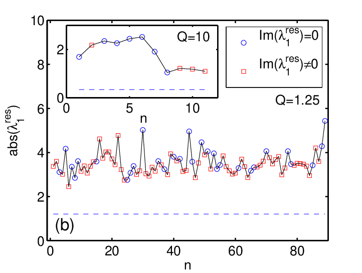
In this section we discuss the time-dependence of the correlation matrices. We can immediately use the prediction of the support of the eigenvalue spectra in the complex plane $\mathcal{C}$ to determine a minimum sampling period $T$ (or equivalently a minimum value of $Q$ ) at which the estimated cross-correlations still exhibit non-random structure. This is possible since we know that if eigenvalues are outside the support the data is non-random. Reducing $T$ too much one expects to arrive a very noisy estimate of the lagged correlation matrix, which will manifest itself in having no departing eigenvalues at all.

We calculate ${\bf C}_{1}{}(T_{i})$ for consecutive, non-overlapping time periods $T_{i}$ and find that – very remarkably – down to a information to noise ratio of $Q\approx{}1.25$ , clear deviations from the predicted support occur. This means that even though noise is drastically increased for low values of $Q$ , non-random structures prevail even at short time-scales.

More specifically, we analyzed 11 correlation matrices obtained from time slices of $4000$ observations (Q=10), and 89 matrices for $500$ time points each. For each individual sub-period $T_{n}$ , we compute lagged correlation matrices ${\bf C}(T_{n})$ for the raw data as well as on the matrices resulting from the regression model, ${\bf C^{res}}(T_{n})$ . Figure 10 (a) shows a plot of the absolute value, $\mathrm{abs}(\lambda_{n})$ , of the maximal eigenvalue found for each sub-period, indexed by $n$ . The dashed blue line corresponds to the prediction of the support $r_{max}$ . We immediately recognize that for $Q=10$ , as well as for $Q=1.25$ the largest eigenvalue lies significantly above the noise regime. On the other hand, the absolute value of the largest eigenvalue is quite volatile and anti-persistent for $Q=1.25$ . We also observe that the largest eigenvalues with non-zero imaginary parts (red squares) mainly occur at low values of $\mathrm{abs}(\lambda_{n})$ , whereas real eigenvalues occur at absolute values. If the eigenvalue is real, the lead-lag network is dominated by strong, approximately symmetric effects; for imaginary eigenvalues the network is dominated by asymmetric correlations, i.e. anti-correlations may play a distinctive part too. We find that if an eigenvalue $\lambda_{1}$ was real (i.e. marked by a blue circle in Fig. 10), the analysis of the preceding sections always identified the IT sector mainly contributing to $\vec{u}_{1}$ (for $Q=10$ ). On the other hand, if the largest eigenvalue was imaginary, no unique interpretation appeared to be valid for all of the sub-periods.

In Fig. 10 (b) we show the same for our continuing antagonist ${\bf X^{res}}$ . Again, we observe $\mathrm{abs}(\lambda_{n})$ being clearly located above the random frontier for all sub-periods. The movement of $\mathrm{abs}(\lambda_{1})$ is less volatile. Closer investigation of the underlying eigenvalues for $Q=10$ revealed changing participation of the sectors (measured by the quantity $I_{si}$ as defined in Eq. (23)). In effect, for all of the 11 sub-periods either the Energy (in periods 6-9) or the Utilities sector (in periods 3, 5) appeared as primarily contributing. In the rest of the periods, both of these sectors were represented strongly in $I_{si}$ .

The last question addressed in this analysis is about the correlations of the lagged correlation matrices: Are significant lagged correlations only found a posteriori or does the data indicate a possibility for a reasonable prediction of future lead-lag structures? To this end we calculate the correlation of matrix elements between the lagged correlation matrices obtained from different (non-overlapping) observation periods $T_{n}$ and $T_{m}$ ,

\begin{split}&c(T_{n},T_{m})=\\ &\frac{\langle{(C^{ij}_{\tau}(T_{n})-\langle{}C^{ij}_{\tau}(T_{n})\rangle_{ij})(C^{ij}_{\tau}(T_{m})-\langle{}C^{ij}_{\tau}(T_{m})\rangle_{ij})}\rangle_{ij}}{\sigma_{T_{n}}\sigma_{T_{m}}}\quad.\end{split}

(25)

Here, the average extends over all matrix-elements and $\sigma_{T_{n}}$ denotes the standard deviation of matrix ${\bf C}_{1}(T_{n})$ . Figure 11 depicts the characteristics we obtained from empirical data. While the expected band of correlation-coefficients would be bound by very small values (in the order of $1/400$ ), we find extremely significant correlations, especially for the $Q=10$ case. As expected, the ’predictability’ of future weighted lead-lag matrices is significantly higher for lagged matrices calculated over longer sub-periods. The inset of Figure 11 shows $c^{\rm res}(T_{n},T_{m})$ , i.e. the same quantity calculated for the residual data. Overall correlations are lower in this case, meaning nothing else than that the market-wide movements exhibit predictable lead-lag structures. However, note that for Q=10 the fluctuations of $\mathrm{abs}(\lambda_{n})$ depicted in the inset of Fig. 10 are not mirrored by any specific variation of $c(T_{1},T_{1}+d)$ in Fig. 11.

Although the present analysis of time-dependence is not comprehensive in every respect, we may state that non-random structures prevail to quite low information-to-noise ratios and that a significant amount of lagged correlation matrices is predictable for future periods. However, shortening the length of the sub-periods results in decreasing predictability.

V Conclusion

We have applied random matrix theory to lagged cross-correlation matrices and theoretically derived the eigenvalue spectra emanating from the respective real asymmetric random matrices in dependence of the information to noise ratio, $Q$ . Specifically, we have shown that – in the case of any eigenvalue ’gas’ satisfying circular symmetry – an inverse Abel-transform can be used to reconstruct the radial density, $\rho(r)$ , from rescaled projections available via solutions of the symmetrized problem. Based on these theoretical results, we analyzed empirical cross-correlations of 5 min returns of the S&P500. For the full time-period observed, we found remarkable deviations from the prediction of the efficient market hypothesis and discussed various structural properties of these deviations. We found the largest eigenvalue being associated with a sub-matrix of exponentially distributed entries. This eigenvalue was associated with a strong hub-like leading influence of the IT sector. Analyzing data based on the residuals of a regression to common movements, we found that cluster structure in the lead-lag network is strongly enhanced. Looking at lagged correlation matrices pertaining to sub-periods of the overall investigation period we found that deviations from the theoretical prediction do occur at quite low information to noise ratios. We also found that significant parts of the lagged correlation matrix should be predictable via measurements of past (non-overlapping) periods.

We think that the current work can be extended in various directions. On the theoretical side, a closer investigation of the nature finite-size effects in the ensemble of time-lagged correlation matrices and comparison with the exact finite-size result of the random real asymmetric case edelman would be tempting. Finite-size effects could also be inferred from the terms which were found to vanish in the $N\rightarrow{}\infty$ limit in Appendix A. We also think that some work is needed in an exact understanding of the relation between the eigenvalue spectra (including the left and right eigenvectors of the ensemble discussed here) and the singular value decomposition of related problems Bouchaud. Also a rigorous study of a ’cleaning procedure’ along the lines of methods already worked out for equal-time financial covariance matrices could be pursued as well.

Finally we believe that the presented work – in general – should allow for an eigenvalue-dependent, systematic study of the influence of matrices and their interplay with equal time-correlations between financial assets in concrete models. The fact that cluster structure conforming with market sectors can be found in lagged correlation matrices already indicates the direction of findings to be expected from such work.

Acknowledgements

We thank J.D. Farmer for encouraging discussions on the matter and Jean-Phillipe Bouchaud for various very useful suggestions, especially for pointing out Eq. (11) to C.B., who further acknowledges useful information from M. Biely. Data is by courtesy of red-stars.com data AG, the paper was sponsored in part by the Austrian Science Fund under FWF project P17621-G05.

Appendix A

Based on the series expansion (11) of the potential $\phi$ , we have calculated the first four terms in the series. For the first term, one easily obtains

\lim_{N\rightarrow\infty}\frac{1}{N}\langle\mathrm{Tr}(B)\rangle{}_{c}=\lim_{N\rightarrow\infty}\frac{1}{N}\mathrm{Tr}(\langle{}C^{ij}C^{ji}\rangle{}_{c})=\frac{1}{Q}\quad.

(26)

since all other terms vanish as $\mathrm{Tr}(C)$ gives just $N$ times the averages of the autocorrelation of the assumed iid white noise process. For calculating the second term, it is useful to remember $\mathrm{Tr}(\mathbf{A}\mathbf{B})=\mathrm{Tr}(\mathbf{B}\mathbf{A})$ and $\mathrm{Tr}({\bf C}{\bf C})=\mathrm{Tr}({\bf C}^{T}{\bf C}^{T})$ as well as taking into account that odd powers of $C$ vanish. One then arrives at

\begin{split}\lim_{N\rightarrow\infty}\frac{1}{N}\langle\mathrm{Tr}(B^{2})\rangle{}_{c}&=\lim_{N\rightarrow\infty}\frac{1}{N}(\mathrm{Tr}(\langle{}(C^{ij}C^{ji})^{2}\rangle{}_{c})\\ &+(x^{2}+y^{2})\mathrm{Tr}(\langle{}2C^{ij}C^{ji}\rangle{}_{c})\\ &+(x^{2}-y^{2})\mathrm{Tr}(\langle{}2C^{ij}C^{ij}\rangle{}_{c}))\quad.\end{split}

(27)

This structure is also typical for higher order terms (not shown for brevity). The trace in the ’dangerous’ term proportional to $x^{2}-y^{2}$ is nothing else than $N$ times the variance of autocorrelations which is just $1/T$ for a Gaussian process. Thus, in total, the term vanishes as $1/T$ in the limit $N\rightarrow\infty$ with $Q=\mathrm{const.}$ , and one gets

\lim_{N\rightarrow\infty}\frac{1}{N}{\mathrm{Tr}\langle{}(B^{2})\rangle{}_{c}}=K+2rQ^{-1}\quad.

(28)

In very similar calculations, it is easy (but tedious), to check that

\begin{split}\frac{1}{N}\langle\mathrm{Tr}(B^{3})\rangle{}=f(r)\quad\mathrm{and}\quad\frac{1}{N}\langle\mathrm{Tr}(B^{4})\rangle{}=g(r)\quad.\end{split}

(29)

The typical situation for higher order terms is similar to the one for the second order term, i.e. the terms in $r$ generally depend on some function of $Q$ and the ’dangerous’ terms (like $(x^{2}-y^{2})^{2}$ ) vanish since they remain constant for growing matrix size and are thus neutralized by the prefactor $1/N$ . We do not expect any different behavior for terms higher than fourth order.

Appendix B

The uniform eigenvalue distribution of real asymmetric matrices in the complex plane $\mathcal{C}$ found in crisantisommers can be almost trivially recovered from Wigner’s semicircle law of real symmetric matrices via application of the inverse Abel-transform. Starting from Wigner’s semicircle law $\rho(\bar{\lambda})=\frac{1}{2\pi}\sqrt{4-\bar{\lambda}^{2}}$ and after proper rescaling $\rho_{x}(\lambda)=\frac{1}{\sqrt{2}\pi}\sqrt{4-2\lambda^{2}}$ we may insert into Eq. (16) and arrive at

\begin{split}\rho(\lambda)&=\frac{1}{\pi^{2}}\int_{r}^{\sqrt{2}}\frac{\lambda}{\sqrt{2-\lambda^{2}}\sqrt{y^{2}-\lambda^{2}}}\mathrm{d}\lambda\\ &=\frac{1}{\sqrt{2}\pi^{2}}\mathrm{arctan}\left(\frac{\sqrt{2-\lambda^{2}}}{\sqrt{\lambda^{2}-r^{2}}}\right)\Bigg|_{r}^{\sqrt{2}}=\frac{1}{2\pi}\quad.\\ \end{split}

(30)

We immediately arrive at the result of an uniform eigenvalue distribution,

\rho(r)=\left\{\begin{array}[]{cc}\frac{1}{2\pi}&0<r<\sqrt{2}\\ 0&\mathrm{elsewhere}\end{array}\right.\quad.

(31)

Appendix C

For $Q=1$ , one solution can be written in the form

G^{H}_{r=1}(z)=\frac{1}{\sqrt{2}}\sqrt{1-\frac{\sqrt{z^{2}-4}}{z}}\quad.

(32)

Note, that this equation shows a simple relation to the resolvent of the Gaussian orthogonal ensemble ( $G^{S}_{Q=1}=\sqrt{\frac{1}{z}G^{GOE}_{r=1}(z)}$ ). The eigenvalue spectrum following from Eqs. (14) and (32) can then be written as

\begin{split}\rho^{Q=1}(\bar{\lambda})=&\frac{1}{\sqrt{2}\pi}\frac{\sqrt{-\frac{1}{2}+\frac{2}{2+|\bar{\lambda}|}}}{\sqrt{\frac{|\bar{\lambda}|}{2+|\bar{\lambda}|}}}\\ =&\frac{1}{\sqrt{2}\pi}\sqrt{-\frac{1}{2}-\frac{1}{|\bar{\lambda}|}+\frac{2}{2+|\bar{\lambda}|}+\frac{4}{|\bar{\lambda}|(2+|\bar{\lambda}|)}}\quad,\end{split}

(33)

and is valued on the support $\left[-2,2\right]$ . After proper rescaling and taking an expression equivalent to Eq. (16), namely

\rho^{Q=1}(r)=-\frac{1}{\pi{}r}\frac{\mathrm{d}}{\mathrm{d}r}\int_{r}^{\infty}{}\lambda\frac{\rho_{x}^{Q=1}(\lambda)}{\sqrt{\lambda^{2}-r^{2}}}\mathrm{d}\lambda\quad,

(34)

we end up with the expression

\rho^{Q=1}(r)=-\frac{1}{\pi{}^{2}r}\frac{\mathrm{d}}{\mathrm{d}r}\int_{r}^{\sqrt{2}}\frac{\lambda\sqrt{\frac{\sqrt{2}}{\lambda}-1}}{\sqrt{\lambda^{2}-r^{2}}}\mathrm{d}\lambda\quad,

(35)

which can be evaluated to

\begin{split}\rho^{Q=1}(r)&=\frac{1}{K}\left[2^{3/4}{}3{}r\Gamma\left(\frac{5}{4}\right)\Gamma\left(\frac{5}{4}\right)\Phi_{2}^{1}\left(\frac{1}{4},\frac{5}{4},\frac{3}{2},\frac{\lambda^{2}}{2}\right)\right.\\ &\left.-2^{1/4}\Gamma\left(-\frac{1}{4}\right)\Gamma\left(\frac{7}{4}\right)\Phi_{2}^{1}\left(-\frac{1}{4},\frac{3}{4},\frac{1}{2},\frac{\lambda^{2}}{2}\right)\right]\quad,\end{split}

(36)

where $K=6\sqrt{\pi^{5}{}r^{3}}$ , $\Gamma(x)$ denotes the Gamma-Function and $\Phi_{2}^{1}(a,b,c,x)$ is the hypergeometric function. It can be checked, that – of course – $\int_{0}^{\sqrt{2}}2\pi{}r\rho(r)\mathrm{d}r=1$ .

References

(1) W. F. Sharpe, Capital Asset Prices: A Theory of Market Equilibrium Under Conditions of Risk, Journal of Finance 19, 425-442 (1964).
(2) H. M. Markowitz, Portfolio selection Journal of Finance 7, 77-91 (1952).
(3) L. Laloux, P. Cizeau, J.-P. Bouchaud, M. Potters, Noise Dressing of Financial Correlation Matrices, Phys. Rev. Lett. 83, 1467 (1999).
(4) V. Plerou, P. Goprikrishnan, B. Rosenow, L. A. N. Amaral, H.E. Stanley, Universal and Nonuniversal Properties of Cross Correlations in Financial Time Series, Phys. Rev. Lett. 83, 1471 (1999).
(5) V. Plerou, P. Gopikrishnan, B. Rosenow, L. A. N. Amaral, T. Guhr, H. E. Stanley Random matrix approach to cross correlations in financial data, Phys. Rev. E 65, 066126 (2002).
(6) D.-H. Kim, H. Jeong, Systematic analysis of group identification in stock markets Phys. Rev. E 72, 046133 (2005).
(7) M. Potters, J. P. Bouchaud, L. Laloux, Financial Applications of Random Matrix Theory: Old Laces and New Pieces, Acta Physica Polonica B 36, 9 (2005).
(8) E. P. Wigner, Characteristic Vectors of Bordered Matrices with Infinite Dimensions, Ann. Math 62 548 (1955); On the Distribution of the Roots of Certain Symmetric Matrices, Ann. Math 67, 325 (1958).
(9) J. Ginibre, Statistical Ensembles of Complex, Quaternion, and Real Matrices, J. Math. Phys. 6, 440 (1965).
(10) N. Lehmann, H.-J. Sommers, Eigenvalue Statistics of Random Real Matrices, Phys. Rev. Lett. 67, 941 (1991).
(11) A. Edelman, The probability that a Random Real Gaussian Matrix has $k$ Real Eigenvalues, J. Multivariate Anal. 60, 203-232 (1997).
(12) E. Kanzieper, G. Akemann, Statistics of Real Eigenvalues in Ginibre’s Ensemble of Random Real Matrices, Phys. Rev. Lett. 95, 230201 (2005).
(13) J. Wishart, The generalized product moment distribution in samples from a normal multivariate population, Biometrika 20 32 (1928).
(14) A. Utsugi, K. Ino, M. Oshikawa, Random matrix theory analysis of cross correlations in financial markets, Phys. Rev. E 70, 026110 (2004).
(15) K. B. K. Mayya and R. E. Amritkar, Delay correlation Matrices, cond-mat/0601279 (2006).
(16) Z. Burda, A. Jarosz, J. Jurkiewicz, M. A. Nowak, G. Papp, I. Zahed, Applying Free Random Variables to Random Matrix Analysis of Financial Data, cond-mat/0603024 (2006).
(17) A. W. Lo, A. C. MacKinlay, When are contrarian profits due to stock market over-reaction?, Review of Financial Studies 3, 175-206 (1990).
(18) T. Chordia, B. Swaminathan, Trading volume and cross-autocorrelations in stock returns Journal of Finance 55, 913-936 (2000).
(19) K. Chan, Imperfect information and cross-autocorrelation among stock prices, Journal of Finance 48, 1211-1230 (1993).
(20) M. J. Brennan, N. Jegadeesh, B. Swaminathan, Investment analysis and the adjustment of stock prices to common information, Review of Financial Studies 6, 799-824 (1993).
(21) S. G. Badrinath, J. R. Kale, T.H. Noe, Of shepherds, sheep, and the cross-autocorrelations in equity returns, Review of Financial Studies, 8, 401-430 (1995).
(22) A. Hameed, Time-varying factors and cross-autocorrelations in short-horizon stock returns, Journal of Financial Research 20, 435-458 (1997).
(23) R. Mench, Portfolio return autocorrelation, Journal of Financial Economics 34, 307-344 (1993).
(24) J. Boudoukh, R. Richardson, R. Whitelaw, A tale of three schools: Insights on autocorrelation of short-horizon returns, Review of Financial Studies 7, 539-573 (1994).
(25) D. Bernhardt, R. J. Davies, Portfolio cross-autocorrelation puzzles, Working Paper (2005)
(26) L. Kullmann, J. Kertesz, K. Kaski, Time dependent cross correlations between different stock returns: A directed network of influence, Phys. Rev. E 66, 026125 (2006).
(27) T. W. Epps, Comovements in stock prices in the very short run, Journal of the American Statistical Association 74, 291-298 (1979).
(28) B. Toth, J. Kertesz, Increasing market efficiency: Evolution of cross-correlations of stock returns, Physica A 360, 505 (2006).
(29) R. A. Janik, M. A. Nowak, G. Papp, J. Wambach, I. Zahed, Non-Hermitian random matrix models: Free random variable approach, Phys. Rev. E 55, 4100-4106 (1997).
(30) H. J. Sommers, A. Crisanti, H. Somopolinsky, Y. Stein, Spectrum of Large Random Asymmetric Matrices, Phys. Rev. Lett. 60, 1895 (1988).
(31) J. P. Bouchaud, private communication (2006).
(32) V. L. Girko, Spectral Theory of Random Matrices (in Russian), Nauka, Moscow (1988).
(33) P. J. Forrester, Log-gases and random matrices, in preparation, www.ms.unimelb.edu.au/ matpjf/matpjf.html
(34) R. Bracewell, The Fourier transform and its Applications, McGraw-Hill, New York (1965).
(35) J. Feinberg, R. Scalettar, A. Zee, ’Single ring theorem’ and the disk-annulus phase transition, J. Math. Phys. 42, 5718 (2001).
(36) J. P. Bouchaud, L. Laloux, M. M. Augusta, M. Potters, Large dimension forecasting models and random singular value spectra, physics/0512090 (2005).
(37) J. P. Bouchaud, M. Potters, Theory of Financial Risk, Cambridge University Press, Cambridge (2000).
(38) P. Cizeau, J. P. Bouchaud, Theory of Levy matrices, Phys. Rev. E 50, 1810 (1994).
(39) Z. Burda, R. A. Janik, J. Jurkiewicz, M. A. Nowak, G. Papp, I. Zahed Free random Levy matrices, Phys. Rev. E 65, 021106 (2002).
(40) R.N. Mantegna, Hierarchical structure in financial markets, Eur. Phy.s. J. B 11, 193-197 (1999).
(41) T. J. Asaki, R. Chartrand, K. R. Vixie, B. Wohlberg, Abel inversion using total-variation regularization, Inverse Problems 21, 1895-1903 (2005).