Convective Patterns in Binary Fluid Mixtures with Positive Separation Ratios

We consider a horizontal layer of a binary fluid mixture of thickness $d$ in a homogeneous gravitational field, $\vec{g}=-g\,\vec{e}_{z}$. A vertical temperature gradient is imposed by fixing the temperature

e.g., via highly conducting plates in experiments. Here we consider the plates to be infinitely extended, rigid, and impermeable. $T_{0}$ is the mean temperature of the fluid layer.

In the conductive state a linear temperature profile

is established. If there is a Soret effect, the temperature gradients generate also a concentration gradient:

Here $C$ means the concentration of the lighter component with $S_{\mathrm{T}}$ being its Soret coefficient. We will consider the case of negative $S_{\mathrm{T}}$. In this case the lighter component of the mixture is driven into the direction of higher temperature. Concentration at the bottom is larger in the conductive state for positive $\Delta T$ therefore enhancing the density gradient and further destabilizing the fluid layer.

Convection is described in terms of the fields of $T$, $C$, velocity $\vec{u}=(u,v,w)$, total mass density $\varrho$, and pressure $P$. In the balance equations connecting these fields we scale lengths and positions by $d$, time by the vertical thermal diffusion time $d^{2}/D_{\mathrm{th}}$, temperature by $\nu D_{\mathrm{th}}/\alpha gd^{3}$, concentration by $\nu D_{\mathrm{th}}/\beta gd^{3}$, and pressure by $\varrho_{0}D_{\mathrm{th}}^{2}/d^{2}$. Here $\varrho_{0}$ is the mean density, $D_{\mathrm{th}}$ the thermal diffusivity, $\nu$ the kinematic viscosity, and $\alpha=-(1/\rho)\partial\rho/\partial T$ and $\beta=-(1/\rho)\partial\rho/\partial C$ are thermal and solutal expansion coefficients, respectively. Using the Oberbeck–Boussinesq approximation the balance equations read PL84; HLL92

Here $\theta,c$, and $p$ are the reduced deviations of temperature, concentration, and pressure, respectively, from the conductive profiles.

The Lewis number $Le$ is the ratio of the concentration diffusivity $D$ to the thermal diffusivity $D_{\mathrm{th}}$, therefore measuring the velocity of concentration diffusion. The Prandtl number $Pr$ is the ratio of the momentum diffusivity $\nu$ and $D_{\mathrm{th}}$:

The Rayleigh number $Ra$ measures the thermal driving and the separation ratio $\psi$ measures the strength of the Soret coupling between temperature and concentration fields

We consider here $S_{\mathrm{T}}<0$, i. e. $\Psi>0$ for mixtures with $\alpha,\beta>0$.

The first equation (2.1) expresses the fact that the fluid is considered to be incompressible. (2.1) – (2.1) are the equations of motion for $\vec{u}$, $\theta$ and $c$. The left hand sides of these equations are the substantial time derivatives of the respective fields. The driving forces entering into the momentum balance equation (2.1) are pressure gradients and the buoyancy caused by the temperature and concentration dependence of the density. The remaining term on the right hand side is the momentum diffusion term.

(2.1) and (2.1) contain also diffusion terms on the right hand side. The off-diagonal term $-Le\,\psi\,\nabla^{2}\,\theta\,$ and the term $Ra\,\psi\,w$ in the concentration balance equation (2.1) describe the action of the Soret effect, i.e., the generation of concentration currents and concentration gradients by temperature variations.

The Dufour effect, i.e., the driving of temperature currents by concentration variations is of interest only in gas mixtures HLL92. But even there it is often small LA97.

We are concerned with three-dimensional convection patterns periodic in the $x$- and $y$-direction. To describe such patterns with wavenumbers $k_{x}$ and $k_{y}$ each field $X$ is expanded as

Here $l$ and $m$ are integers and the $f_{n}$ form a complete system of functions that fits the specific boundary condition for the field $X$ at the plates. To find suitable sets of functions $f_{n}$ we introduce some new fields. First, two scalar fields $\Phi$ and $\Psi$ are defined via

The structures we want to discuss do not show a horizontal mean flow for mirror symmetry reasons. Then, (8) is the most general expression that fulfills the incompressibility condition (2.1) CB89.

Second, instead of $c$ we use the field

that allows in a more convenient way to guarantee the impermeability of the horizontal boundaries: The diffusive part of the concentration current, driven by concentration gradients as well as by temperature gradients is given by $-Le\,\nabla(c-\psi\theta)$. At the impermeable plates the vertical component of this current vanishes which requires

The advective concentration current vanishes at the plates because there ${\bf u}=0$. The balance equation for $\zeta$ is obtained by combining (2.1) and (2.1).

The boundary conditions for the fields $\Phi,\Psi,\theta$, and $\zeta$ read

To expand the fields $\Psi$, $\theta,\zeta$, and $\Phi$ vertically we used different orthonormal sets $f_{n}(z)$ as follows

Here $C_{n}$ and $S_{n}$ are Chandrasekhar–Reid functions C81.

The balance equations for the new fields are

Here $\Delta_{2}=\partial_{x}^{2}+\partial_{y}^{2}$.

By inserting the ansatz (7) for each field into the balance equations and projecting them onto the basic functions one gets a nonlinear algebraic system of equations of the form

For simplicity amplitudes are labelled here by a single Greek index and the summation convention is implied in (14) with $A_{\kappa\mu},B_{\kappa\mu}$, and $C_{\kappa\mu\nu}$ being constant coefficients.

The number of modes has to be truncated to get a finite number of equations as discussed later on. For stationary convection structures the left hand side of (14) vanishes and the solution can be found using a multidimensional Newton method.

To make a full stability analysis one has to check the stability of the patterns against perturbations with arbitrary wavevector $d\vec{e}_{x}+b\vec{e}_{y}$. To do so one has to introduce a Floquet term writing out the perturbation as

Such a perturbation is added to the known solution the stability of which is to be tested and inserted into the balance equations. After linearizing and projecting one gets a linear eigenvalue problem of the form

with constant coefficients $A_{\kappa\mu}$ and $B_{\kappa\mu}$. The aforementioned solution, i.e., the convective structure described by it is stable if every eigenvalue $s$ has a negative real part for every $d$ and $b$.

The symmetry of the convective pattern discussed above can under some circumstances be used to get separated classes of possible eigenvectors representing the perturbations. That means the eigenvalue problem can be reduced to finding the eigenvalues of two matrices of about half of the size. Because evaluating the eigenvalues of a matrix is a $O(N^{3})$-process this always implies a reduction of the computation time.

In pure fluids convection in the Rayleigh--Bénard system starts at a critical Rayleigh number $Ra_{\mathrm{c}}^{0}=Ra_{\mathrm{c}}(\psi=0)=1707.762$ and a wavenumber $k_{\mathrm{c}}^{0}=k_{\mathrm{c}}(\psi=0)=3.117$ C81. In binary mixtures with positive separation ratios that we are dealing with, the critical Rayleigh number is smaller, $Ra_{\mathrm{c}}(\psi>0)<Ra_{\mathrm{c}}^{0}$, since the solutal contribution to the quiescent state’s buoyancy force enhances the latter. Thus a smaller thermal driving, i.e., a smaller Rayleigh number suffices to reach the critical buoyancy force size for onset of convection. The critical wavenumber is also somewhat lower: $k_{\mathrm{c}}(\psi>0)<k_{\mathrm{c}}^{0}$ KM88. When presenting our results we shall use the reduced Rayleigh number

The convection above onset depends on the three parameters $\psi$, $Le$, and $Pr$. These parameters depend on the components of the mixture and the mean values of temperature and concentration. For alcohol-water for example, $\psi$ may assume values between $-0.6$ and $0.3$. Here the Lewis number $Le=0.01$ or smaller whereas $Le\approx 1$ is typical for gas mixtures. A typical Prandtl number for liquid mixtures is $Pr=10$, in gas mixtures $Pr=0.1$…$1$.

Calculating the fixed point solutions and analyzing their stability requires less numerical effort than for 3D structures. Only $X_{l0n}$-modes have to be taken into account and $\Psi\equiv 0$. Mirror symmetry in the lateral direction allows to set $X_{l0n}=X_{-l0n}$ so that the lateral functions $\mathrm{e}^{\pm{\rm i}klx}$ can be replaced by $\cos(klx)$. In addition the roll pattern is antisymmetric under reflection at the plane $z=0$ combined with a translation by half a wavelength in $x$-direction. This mirror glide symmetry enforces half of the amplitudes to be zero, e. g. all amplitudes $\Phi_{l0n}$ where $l+n$ is an odd number.

To perform the stability analysis of rolls one determines the growth behavior of perturbations of the form

Because of the periodicity of the patterns in $x$ and its mirror symmetry it suffices to consider $d\in\left[0,k/2\right]$. In $y$-direction, however, all perturbation wavenumbers, say, $b\geq 0$ have to be investigated. For a discussion of the effect of mean flow perturbations, e. g., $\delta\Phi_{00n}$ we refer to HLBJ00.

The linear system of equations (18) always separates into two subsystems of perturbations $\delta X_{l0n}$ that belong to modes with amplitudes $X_{l0n}$ that are antisymmetric or symmetric under the mirror glide operation $(x,z)\rightarrow(x+\lambda/2,-z)$. E. g. all perturbations with amplitudes $\delta\Phi_{l0n}$ with even $l+n$ belong to one set, while the perturbations with odd $l+n$ belong to the other.

In special cases the system of equations can be separated even further. For $d=0$ the perturbations can be divided into those that are symmetric and those that are antisymmetric under the operation $x\rightarrow-x$. Furthermore, if $b=0$ then the perturbations contain either no or only $\delta\Psi$-amplitudes. This is also of practical interest, since some instabilities are most critical in these special cases.

The sets of modes taken into account in the Galerkin procedure were chosen as follows: We defined a maximal mode index $N$ and neglected all modes $X_{l0n}$ or $\delta X_{l0n}$ with $|l|+n>N_{1}$ for $\Phi$- and $\Psi$-fields and $|l|+n>N_{2}$ for $\theta$- and $\zeta$-fields. Here $N_{2}=2N_{1}$.

A quantitative description of the fixed point solutions and the stability behavior in binary mixtures requires in some cases sets of modes that are much larger than those needed for pure fluids. This is because the strong anharmonic narrow boundary layer behavior of the $\zeta$-field for small $Le$ and large $r$. For the most anharmonic roll structures at $r\approx 1.5$, $Le<0.01$, and $\psi=0.15$ that we have investigated expansions up to $N_{2}=40$ were needed. Although the velocity and temperature field are much smoother, a consistent description of the latter requires then also high $\theta$-modes as discussed in HL98; H96. This is much more than for pure fluids, where truncations with $N\leq 8$ are sufficient to describe the stability behavior quantitatively even at large $r$.

We will discuss the fixed point solutions by focusing on the mode intensity $|\Phi_{101}|^{2}$ at $k=k^{0}_{\mathrm{c}}$ as order parameter (see Fig. 1). The relation to the vertical velocity $w$ is $k^{2}\Phi_{101}=w_{101}$. It is useful to start with considering solutions for small $Le$. In this case, two different convection regimes can be distinguished. For $r<1$, in the Soret regime, the applied temperature gradients cause convection only indirectly, by generating concentration and therefore density gradients via the Soret effect. The convection amplitudes are very small here. This changes in the Rayleigh regime, where the temperature gradients cause the necessary density gradients to develop convection also directly. $|\Phi_{101}|^{2}(r)$ strongly curves upward and $|\Phi_{101}|^{2}$ assumes values comparable to those of pure fluid convection, since concentration is more and more equilibrated.

The transition between Soret and Rayleigh region is especially sharp if $\psi$ is also small. It is also present for larger $Le$, but more smooth. It vanishes for $Le\approx 1$. The knowledge of these features will be helpful for a qualitative understanding of the stability behavior.

The stability boundaries of roll patterns in pure fluids are known since the pioneering work of Busse and his coworkers B78. At small Rayleigh numbers there exist five different instability mechanisms giving rise to five different stability boundaries that limit the region of stable rolls in the $(Ra,k,Pr)$-parameter space. At small Prandtl numbers the Eckhaus (EC), the skewed varicose (SV), and the oscillatory mechanism (OS) are the important instabilities CB90. At higher Prandtl numbers the zigzag (ZZ) and the crossroll (CR) mechanisms dominate B67. Properties and symmetries of these perturbations are discussed in BBC85. These five instabilities of roll patterns are the same as those that can be found in binary mixtures. A more detailed discussion of the symmetries and other features of these mechanisms can be found in HLBJ00.

The central qualitative difference between roll structures in pure fluids and binary mixtures concerning their stability is certainly their loss of stability in mixtures at onset in a wide range of parameter space. However, roll structures do in general still exist in mixtures as stable structures for these parameters, not at onset, but at larger $r$. Figure 2 shows the CR instability boundaries of rolls in a parameter interval where an exchange of stability between rolls and squares at onset is predicted in ClK91. One sees that the curvature of the CR boundary at the critical point diverges – a feature that follows also from cubic amplitude equations, see HLBJ00 – when this exchange occurs. For the parameters $Pr=10,\psi=0.01$ of Fig. 2 the exchange occurs at $Le=0.2$. Decreasing $Le$ below this value the neutral stability curve (dashed line in Fig. 2) drops further down in $r$ (not shown in Fig. 2b) while the CR instability boundary disconnects from the neutral stability curve and moves up in $r$. Above the CR boundary rolls are still stable against CR perturbations.

The rolls could still be unstable there against other perturbations but we found the minimum of the CR boundary always to be the minimal Rayleigh number above which stable rolls exist. Only at $\psi=0.15$, $Pr<0.2$ and $Le<0.015$ we found regions where rolls seem to be unstable everywhere in the $(k,r)$-plane. The two branches of the CR boundary meet again at higher $r$ near this region and limit an oval region of CR-stable rolls from below and also above. The oval region gets smaller by reducing $Le$ or $Pr$ until the region of stable rolls vanishes. The experimental observation of this behavior might be difficult because it occurs in a region of the parameter space that is not accessible by ordinary fluid mixtures.

We have calculated all stability boundaries at small $r$ for different values of $Le$, $\psi$, and $Pr$. Concerning the stability behavior of the roll structures one sees that in the Rayleigh region, $r>1$, where the concentration field is nearly uniform the binary mixture behaves like a pure fluid. As for the fixed points, the transition between Soret and Rayleigh region is very sharp at small $Le$ and $\psi$. An example for such a behavior is given in Fig. 3. Here only the EC, CR, and ZZ boundaries are of importance. In the Rayleigh region of Fig. 3 the CR, ZZ, and EC boundaries of the mixture (full lines with circles, triangles, and squares, respectively) are lying close to the corresponding boundaries of the pure fluid (long-dashed lines). Note in particular the vase-like form of the EC boundary $r_{\mathrm{EC}}(k)$ and the dent in the ZZ boundary $r_{\mathrm{ZZ}}(k)$: Closer to onset ($r_{\mathrm{c}}\simeq 0.6,k_{\mathrm{c}}\simeq 2.6$ in Fig. 3), i.e., in the Soret regime $r_{\mathrm{EC}}(k)$ opens up parabolically and $r_{\mathrm{ZZ}}(k)$ comes out of the critical point linearly with positive slope. However, in the crossover range $r\sim 1$ between Soret and Rayleigh regime the curve $r_{\mathrm{EC}}(k)$ pinches inwards and develops a waist such as to follow in the Rayleigh regime the parabolic shape of the EC curve of the pure fluid that starts out at $k_{\mathrm{c}}^{0}\simeq 3.1,r_{\mathrm{c}}^{0}=1$. Similarly $r_{\mathrm{ZZ}}(k)$ bends in the crossover range towards small $k$ to follow then the ZZ boundary of the pure fluid that shows negative slope.

Figure 4 show that this transition between Soret and Rayleigh region that causes the vase-like structure of the EC boundary and the sharp bend of the ZZ boundary is smoother for larger $Le$ or $\psi$. For $Le=1$, the stability balloon does not qualitatively differ from its pure fluid counterpart.

Squares have the same symmetry plane at $x=0$ as rolls and an additional mirror plane at $y=0$. Furthermore, squares show also a mirror glide symmetry. Here, however, the symmetry transformation consists of a reflection at the plane $z=0$ combined with a translation by half a wavelength in $x$- and $y$-direction. To describe these three-dimensional patterns the $\Psi$-field cannot be neglected. We also mention that in contrast to the other fields $\Psi$ is odd in $x$ and $y$ and has positive parity under the mirror glide operation thereby reflecting the symmetries of the velocity field. A further reduction of the number of mode occurs since square patterns are invariant under rotation by $90^{\circ}$ mapping the $x$- onto the $y$-directions and vice versa. Amplitudes like $\Phi_{lmn}$ and $\Phi_{mln}$ are the same. This is also true for $\theta$ and $\zeta$. Again $\Psi$ is different. Here $\Psi_{lmn}=-\Psi_{mln}$.

Because the amount of computational power needed to make a full stability analysis of these three-dimensional structures is too large, we will discuss perturbations only for periodic boundary conditions, i. e., $d=b=0$. Here again a separation of perturbations is possible into those that change sign or not under the mirror glide operation. Furthermore, the stability problem is invariant under $x\rightarrow-x$ and $y\rightarrow-y$. Thus one can distinguish between perturbations that are even in $x$ and $y$, odd in $x$ and $y$, or even in $x$ and odd in $y$ (or equivalently odd in $x$ and even in $y$). If the perturbations have the same symmetry in both directions one can in the case of squares finally make use of a last symmetry property and separate between perturbations that are symmetric or antisymmetric under the exchange of the $x$- and $y$-direction.

The modes taken into account for the Galerkin procedure were chosen in a way analogous to the roll case: $X_{lmn}$ and $\delta X_{lmn}$ were neglected, if $|l|+|m|+n$ was larger than $N_{1}$ or $N_{2}$ respectively. Since square structures are stable mainly below $r=1$ and the boundary layers are less narrow compared to the coexisting roll solutions (see below), values of $N_{2}\leq 20$ were sufficient.

The convection patterns of squares resemble linear superposition of two perpendicular sets of rolls. The intensities of the leading modes $\Phi^{\mathrm{S}}_{101}=\Phi^{\mathrm{S}}_{011}$ of the square solutions show qualitatively the same $r$-dependence as $\Phi^{\mathrm{R}}_{101}$ for roll solutions but are always smaller. Arguments based on amplitude equations show however, that $|\Phi^{\mathrm{S}}_{101}|^{2}+|\Phi^{\mathrm{S}}_{011}|^{2}>|\Phi^{\mathrm{R}}_{101}|^{2}$ near onset if and only if squares are stable there. But this is no longer true at higher $r$ where the solutions are such that $|\Phi^{\mathrm{S}}_{101}|^{2}+|\Phi^{\mathrm{S}}_{011}|^{2}<|\Phi^{\mathrm{R}}_{101}|^{2}$. This change takes place before squares lose stability.

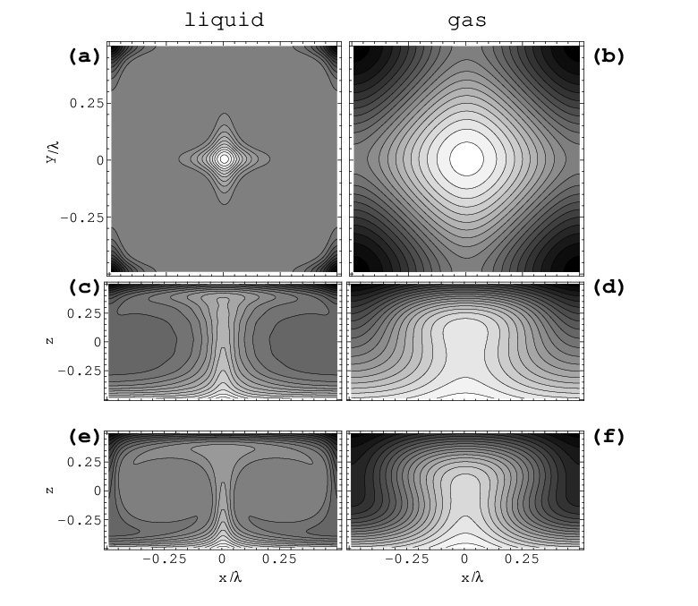
In Fig. 5 we show the concentration distribution of square convection for two parameter combinations that are representative for liquid and gas mixtures. This plot and the concentration field structure of rolls and squares in a vertical cross section shows a characteristic boundary layer and plume behavior at small $Le$. Such structures occur when advective mixing is large compared to diffusion in the bulk of the fluid. Consequently the boundary layers and plumes are more pronounced in rolls than in squares since the leading velocity amplitudes are greater for the former. Thus squares with their broader boundary layers are much smoother structures than rolls at the same parameters. The practically harmonic velocity and temperature fields are not shown.

Performing the stability analysis of squares we had to restrict ourselves to the case $d=b=0$ where the perturbations separate into different symmetry classes. Because both squares and rolls can be described as even in $x$ and $y$ and as mirror glide antisymmetric, one expects a perturbation that destabilizes the squares and favors the rolls to fulfill these symmetries, too. However such a perturbation should break the symmetry $x\leftrightarrow y$. We actually always found the most critical perturbation to fall into this symmetry class. Other perturbations that break the mirror symmetry in $x$- or $y$-direction are less critical.

Figure 6 shows typical examples for the stability region of squares. The left and right side of the stability boundaries should not be taken too serious – presumably square structures are destabilized earlier by instabilities with finite $b$ or $d$ that tune the wavenumber and that are not considered here.

Even if squares are stable at onset they always lose their stability against a roll pattern at higher $r$. Furthermore, for certain parameters there does also exist a band of $r$-values where neither squares nor rolls are stable. Therein crossrolls or oscillations appear as stable patterns.

The numerical investigations of the crossroll structures were performed as in the case of squares except that modes like $X_{lmn}$ and $X_{mln}$ could not be identified anymore due to the lack of the $x\leftrightarrow y$ symmetry. For $b=d=0$ instabilities are either mirror glide symmetric or antisymmetric. They are either even or odd in the $x$- and the $y$-direction. We used expansions up to $N_{2}=20$ to investigate these structures. The time-dependent structures were investigated via direct numerical integration of the equations of motion for the modes.

Stationary crossrolls exist at parameters $Pr,L,\psi$ if squares are stable at onset. Then, they appear in the $r$-range were squares are already and rolls are still unstable. Oscillatory crossrolls exist only at small $Le$. The connection between the different structures can be extracted from the bifurcation diagram in Fig. 7. For the parameters $Pr=27$, $Le=0.0047$, and $\psi=0.23$ taken from MS91, all four kinds of patterns exist. For the calculation of the fixed points a model with $N_{2}=10$ was used, the bifurcation diagram is therefore only qualitatively correct at higher $r$.

We will first ignore the crossroll solutions of the oscillatory type and concentrate on the stationary patterns. At onset squares with $|\Phi_{101}|^{2}=|\Phi_{011}|^{2}$ are the stable structure. The coexisting roll branch is unstable. At about $r=1.11$ a new type of solutions bifurcates out of the square branch, the stationary crossrolls. In this $r$-range neither squares nor rolls are stable. For the crossroll structures the two important mode intensities are different, say $|\Phi_{101}|^{2}>|\Phi_{011}|^{2}$. The difference between these intensities grows until $|\Phi_{011}|^{2}=0$ and $|\Phi_{101}|^{2}$ touches the roll branch at another bifurcation point at $r\approx 1.24$. The crossrolls transfers their stability to the rolls here.

The stationary crossrolls exist always inside an intermediate $r$-range if squares are stable at onset. The oscillatory type appears only at very small $Le$ as in Fig. 7. If these solutions are absent, the squares transfer their stability directly to the stationary crossroll branch, leading to a sequence squares -- stationary crossrolls -- rolls of stable structures for increasing $r$. In particular, the stability boundaries that limit the region of stable squares in Fig. 6 are all of the type leading to stationary rolls: oscillatory crossrolls do not exist for these parameters.

But for the parameters in Fig. 7 the bifurcation behavior is more complicated. The squares lose their stability already at $r\approx 1.08$ before the stationary crossrolls emerge. At this point oscillatory crossrolls grow out of the square state in a supercritical Hopf bifurcation. The stationary crossrolls that appear at $r=1.11$ remain unstable until $r\approx 1.14$.

Fig. 8 shows for several Rayleigh numbers that $|\Phi_{101}|^{2}(t)$ and $|\Phi_{011}|^{2}(t)$ oscillate in opposite phase around a common mean value given by the unstable square state. The $x$-roll intensity of the pulsating pattern grows or decreases on cost of the $y$-roll intensity, however, without ever going to zero. Thus the two roll sets never die out completely or reverse their turning direction during the oscillations.

Close to the Hopf bifurcation the oscillations are harmonic and of small amplitude (Fig. 8a). With increasing $r$ the frequency decreases roughly linearly MS91. Furthermore, and more importantly, with increasing amplitude the oscillation becomes more anharmonic and relaxational in Fig. 8b, c; see also Ref. GPC85; MS91: While the system rapidly sweeps through the square state it spends more and more time in the vicinity of the roll state. The change from harmonic in Fig. 8a to strongly relaxational oscillations in Fig. 8c is also documented in the right column of Fig. 8. There we show phase space plots associated with the time histories of $|\Phi_{101}|^{2}$, $|\Phi_{011}|^{2}$ in the left column.

At larger $r$ the system gets attracted into one of the crossroll fixed points that have become stable shortly before oscillatory crossrolls cease to exist in Fig. 7. In this interval we have observed a novel subharmonic bifurcation cascade (SC) in which the crossroll attractors entrain the oscillations: First the crossroll attractors deform the phase trajectory (Fig. 8c). Then with increasing $r$ the oscillations execute an increasing number of windings around the crossroll states. In Figs. 8c – f the winding number around a crossroll fixed point increases from $n$ = 1 to $n$ = 4 and the period $\tau$ of the oscillations increases from $2\pi/\omega$ to $2\pi n/\omega$ in integer steps. This increase of the winding number in the SC continues beyond $n=4$; we have found also $n=5$. However, the control parameter interval $\delta r_{n}$ for an $n$-cycle becomes so narrow – $\delta r_{n}\cong(1.6,0.6,0.2)10^{-4}$ for $n=(2,3,4)$ – that our numerical resources were not sufficient to resolve the SC further. But we think that the SC is a robust, experimentally accessible phenomenon; Ref. GPC85 contains a hint for a 2-cycle. Beyond the SC interval in the system gets attracted into one of the crossroll fixed points. The transition between the oscillations and the crossroll state is slightly hysteretic. Upon reducing $r$ the system remains in the crossroll state until below the SC interval and then a transition to an $n=1$ oscillation occurs. So in a small $r$-interval there is bistable coexistence of oscillations and stationary crossrolls.

References

- (1) M. C. Cross, P. C. Hohenberg: Rev. Mod. Phys. 49, 581 (1993)
- (2) J. K. Platten, J. C. Legros: Convection in Liquids. (Springer, New York 1984)
- (3) M. Lücke, W. Barten, P. Büchel, C. Fütterer, St. Hollinger, Ch. Jung: Pattern formation in binary fluid convection and in systems with throughflow’. In: Evolution of spontaneous structures in continuous systems ed. by F. H. Busse, S. C. Müller. Lecture Notes in Physics 55, 127. (Springer, Berlin, Heidelberg 1998)
- (4) P. Le Gal, A. Pocheau, V. Croquette: Phys. Rev. Lett. 54, 2501 (1985)
- (5) E. Moses, V. Steinberg: Phys. Rev. Lett. 57, 2018 (1986); Phys. Rev. A 43, 707 (1991)
- (6) M. A. Dominguez-Lerma, G. Ahlers, D. S. Cannell: Phys. Rev. A 52, 6159 (1995)
- (7) Ch. Jung, B. Huke, M. Lücke: Phys. Rev. Lett. 81, 3651 (1998)
- (8) S. Chandrasekhar: Hydrodynamic and hydromagnetic stability, Appendix V (Dover, 1981)
- (9) W. Hort, S. Linz, M. Lücke: Phys. Rev. A 45, 3737 (1992)
- (10) J. L. Liu, G. Ahlers: Phys. Rev. E 55, 6950 (1997)
- (11) R. M. Clever, F. H. Busse: J. Fluid Mech. 198, 345 (1989)
- (12) E. Knobloch, D. R. Moore: Phys. Rev. A 37, 860 (1988)
- (13) F. H. Busse: Rep. Prog. Phys. 41, 1929 (1978)
- (14) J. L. Liu, G. Ahlers: Phys. Rev. Lett. 77, 3126 (1996)
- (15) T. Clune, E. Knobloch: Phys. Rev. A 44, 8084 (1991)
- (16) B. Huke, M. Lücke, P. Büchel, Ch. Jung: J. Fluid Mech. 408, 121 (2000)
- (17) St. Hollinger, M. Lücke: Phys. Rev. E 57, 4238 (1998)
- (18) St. Hollinger: Theorie der ausgedehnten stationären und wandernden Konvektion in binären Fluidmischungen. PhD thesis, Universität des Saarlandes, Saarbrücken (1996)
- (19) R. M. Clever, F. H. Busse: Phys. Fluids A 2, 334 (1990)
- (20) F. H. Busse: Journal of Mathematics and Physics 46, 140 (1967)
- (21) E. W. Bolton, F. H. Busse, R. M. Clever: J. Fluid Mech. 164, 469 (1985)