Tomographic inversion using $\mathbf{\ell_{1}}$-norm regularization of wavelet coefficients

Like most geophysical inverse problems, the linearized problem $\mathbf{A}\mathbf{m}=\mathbf{d}$ in seismic tomography is underdetermined, or at best offers a mix of overdetermined and underdetermined parameters. It has therefore long been recognized that it is important to suppress artifacts that could be falsely interpreted as ‘structure’ in the earth’s interior. Not surprisingly, strategies that yield the smoothest solution $\mathbf{m}$ have been dominant in most global or regional tomographic applications; these strategies include seeking global models represented as a low-degree spherical harmonic expansion [Dziewonski et al.(1975), Dziewonski & Woodhouse(1987), Masters et al.(1996)] as well as regularization via minimization of the gradient ($\nabla\mathbf{m}$) or second derivative ($\nabla^{2}\mathbf{m}$) norm of a dense local parametrization [Nolet(1987), Constable et al.(1987), Spakman & Nolet(1988), VanDecar & Snieder(1994), Trampert & Snieder(1996)].

Smooth solutions, however, while not introducing small-scale artifacts, produce a distorted image of the earth through the strong averaging over large areas, thereby making small-scale detail difficult to see, or even hiding it. Sharp discontinuities are blurred into gradual transitions. For example, the inability of global, spherical-harmonic, tomographic models to yield as clear an image of upper-mantle subduction zones as produced by more localized studies has long been held against them. [Deal et al.(1999)] and [Deal & Nolet(1999)] optimize images of upper-mantle slabs to fit physical models of heat diffusion, in an effort to suppress small-scale imaging artifacts while retaining sharp boundaries. [Portniaguine & Zhdanov(1999)] use a conjugate-gradient method to seek the smallest possible anomalous domain by minimizing a norm based on a renormalized gradient $\nabla\mathbf{m}/(\nabla\mathbf{m}\cdot\nabla\mathbf{m}+\gamma^{2})^{\frac{1}{2}}$, where $\gamma$ is a small constant. Like all methods that deviate from a least-squares type of solution, both these methods are nonlinear and pose their own problems of practical implementation.

The notion that we should seek the ‘simplest’ model $\mathbf{m}$ that fits a measured set of data $\mathbf{d}$ to within the assigned errors is intuitively equivalent to the notion that the model should be describable with a small number of parameters. But, clearly, restricting the model to a few low-degree spherical-harmonic or Fourier coefficients, or a few large-scale blocks or tetrahedra, does not necessarily lead to a geophysically plausible solution. In this paper we investigate whether a multiscale representation based upon wavelets [Daubechies(1992)] has enough flexibility to represent the class of models we seek. We propose an $\ell_{1}$-norm regularization method which yields a model $\mathbf{m}$ that has a strong tendency to be sparse in a wavelet basis, meaning that it can be faithfully represented by a relatively small number of nonzero wavelet coefficients. This allows for models that vary smoothly in regions of limited coverage without sacrificing any sharp or small-scale features in well-covered regions that are required to fit the data. Our approach is different from an approach briefly suggested by [de Hoop & van der Hilst(2005)], in which the mapping between data and model is decomposed in curvelets: here we are concerned with applying the principle of parsimony to the solution of the inverse problem, without any special preference for singling out linear features, for which curvelets are probably better adapted than wavelets.

In Section 2 we give a short description of the mathematical method, and in Section 3 we consider a geophysically motivated, toy 2D application, in which the synthetic data are a small set of regional, fundamental-mode, Rayleigh-wave dispersion measurements expressed as wavenumber perturbations $\delta k(\nu)$ at various frequencies $\nu$. To enable us to concentrate on the mathematical rather than the geophysical aspects of the inverse problem, we assume that the fractional shear-velocity perturbations $\delta\hskip-1.00006pt\ln\hskip-1.00006pt\beta=\delta\beta/\beta$ within the region are depth-independent. Finite-frequency interpretation of the surface-wave dispersion data [Zhou et al.(2004)] then yields a 2D linearized inverse problem of the form $\mathbf{A}\mathbf{m}=\mathbf{d}$. We compare wavelet-basis models $\mathbf{m}$ obtained using our proposed $\ell_{1}$-norm regularization with models obtained using more conventional $\ell_{2}$ regularization, both with and without wavelets, and show that the former are sparser and have fewer small-scale artifacts.

In any realistic tomographic problem, the linear system $\mathbf{A}\mathbf{m}=\mathbf{d}$ is not invertible: even when the number of data exceeds the number of unknowns, the least-squares matrix $\mathbf{A}^{T}\mathbf{A}$ is (numerically) singular. Additional conditions always have to be imposed. The proposed regularization method is based on the fundamental assumption that the model $\mathbf{m}$ is sparse in a wavelet basis [Daubechies(1992)]. We believe that this is an appropriate inversion philosophy for finding a smoothly varying model while still allowing for whatever sharp or small-scale features are required to fit the data $\mathbf{d}$. An important feature of the method is that the location of the small-scale features does not have to be specified beforehand.

A wavelet decomposition is a special kind of basis transformation that can be computed efficiently (the number of operations is proportional to the number of components in the input). At each step the algorithm strips off detail belonging to the finest scale present —this detail is encoded in wavelet coefficients, broadly corresponding to local differences— and calculates a coarse version —encoded in scaling coefficients, broadly corresponding to local averages— that is only half the size of the original in 1D and only one quarter the size in 2D. This procedure is repeated on the successive coarse versions. The resulting wavelet coefficients (at the different scales) and scaling coefficients (at the final coarsest scale only) are called the wavelet decomposition of the input. By this construction each wavelet coefficient carries information belonging to a certain scale (by virtue of the decimation) and a certain position (use of local differences). The final few scaling coefficients represent a (very) coarse average.

The mathematical relation between the wavelet-basis expansion coefficients $\mathbf{w}$ and the model $\mathbf{m}$ is the wavelet transform $\mathbf{W}$ (a linear operator): $\mathbf{m}=\mathbf{W}^{T}\mathbf{w}$. By choosing the local differences and averages carefully (corresponding to a choice among many different so-called wavelet families), the inverse transformation from $\mathbf{w}$ back to $\mathbf{m}$ can be made equally efficient. In our application we will use a special kind of 2D wavelet basis that is overcomplete: it contains six different wavelets corresponding to different directions. Because of this overcompleteness, the wavelet transform $\mathbf{W}$ has a left inverse (namely $\mathbf{W}^{T}$): $\mathbf{W}^{T}\mathbf{W}=\mathbf{I}$, but no right inverse, $\mathbf{W}\mathbf{W}^{T}\neq\mathbf{I}$. Appendix B contains a short overview of this particular construction. In short our wavelet and scaling coefficients $\mathbf{w}$ contain information on scale, position and direction.

For the tomographic reconstruction, we will require a sparse set of wavelet-basis coefficients: the vast majority of these represent differences and will only be present around non-smooth features. In this way we regularize the inversion by adapting ourselves to the model rather than to the operator. As a measure of sparsity we will use the $\ell_{1}$-norm of the wavelet representation $\mathbf{w}$ of the model $\mathbf{m}$, i.e. we will look for a solution of the linear equations $\mathbf{A}\mathbf{m}=\mathbf{d}$ that has a small $\|\mathbf{w}\|_{1}=\sum_{i}|w_{i}|$. Since $|w_{i}|>|w_{i}|^{2}$ for small $w_{i}$ and $|w_{i}|<|w_{i}|^{2}$ for large $w_{i}$, this type of penalization will favor a small number of large coefficients over a large number of small coefficients in the reconstruction (whereas a traditional $\ell_{2}$ penalization might do the opposite). We are not claiming that the sparsest solution always coincides with the minimum $\ell_{1}$-norm solution, but one can show that it often does [Donoho(2004), Candes et al.(2006)]. A schematic justification for this is given in Fig. 1.

In particular, our strategy will consist of searching for the minimizer of the functional

where $\tau$ is an adjustable parameter at our disposal. Here, the first (quadratic) term corresponds to the conventional statistical measure of misfit to the data, $\chi^{2}=\sum_{i}[d_{i}-(\mathbf{A}\mathbf{m})_{i}]^{2}$, and the second ($\ell_{1}$-norm) term $2\tau\|\mathbf{w}\|_{1}$ is introduced to regularize the inversion. In writing $\chi^{2}$ in this form, we have made the simplifying assumption that the noisy data $\mathbf{d}$ are uncorrelated with unit variance. More generally, the misfit portion of the functional (1) is $\chi^{2}=(\mathbf{d}-\mathbf{A}\mathbf{m})^{T}\mathbf{\Sigma}^{-1}(\mathbf{d}-\mathbf{A}\mathbf{m})$, where $\mathbf{\Sigma}$ is the data covariance matrix. In the 2D toy problem considered in Section 3, we invert synthetic data $\mathbf{d}$ having a constant (but non-unit) variance, $\mathbf{\Sigma}=\sigma^{2}\mathbf{I}$.

The minimizer of the functional (1) can be found by iteration [Daubechies et al.(2004)]: starting with the present approximation $\mathbf{w}^{(n)}$ one constructs an $n$th-iterate surrogate functional

that has the same value and the same derivative at the point $\mathbf{w}=\mathbf{w}^{(n)}$ as the original functional (see Fig. 2). This surrogate functional can be rewritten as

where $c^{(n)}$ is independent of $\mathbf{w}$. This functional has a much simpler form than the original $I_{1}(\mathbf{w})$ because there is no operator $\mathbf{A}\mathbf{W}^{T}$ mixing different components of $\mathbf{w}$. The next approximation $\mathbf{w}^{(n+1)}$ is defined by the minimizer of this new functional. By calculating the derivative of expression (3) with respect to a specific wavelet or scaling coefficient $w_{i}$, one finds the following set of component-by-component equations:

valid whenever $w_{i}\neq 0$. These equations are solved by distinguishing the two cases $w_{i}>0$ and $w_{i}<0$; the solution —corresponding to the minimizer of the surrogate functional $I_{1}^{(n)}(w)$, and denoted by $\mathbf{w}^{(n+1)}$— is then found to equal

where $S_{\tau}$ is the so-called soft-thresholding operation, i.e.

performed on each wavelet or scaling coefficient $w_{i}$ individually. The starting point of the iteration procedure is arbitrary, e.g. $\mathbf{w}^{(0)}=\mathbf{0}$. Because of the component-wise character of the tresholding, it is straightforward to use different thresholds $\tau_{i}$ for different components $w_{i}$ if desired, and in fact we shall use different thresholds $\tau_{\rm w}$ and $\tau_{\rm s}$ for the wavelet and scaling coefficients in our application. A schematic representation of the idea behind the iteration (5) is given in Fig. 2. We realize that this iteration converges slowly for ill-conditioned matrices, but we use it here because it is proven to converge to the solution [Daubechies et al.(2004)].

An improvement in convergence can be gained by rescaling the operator $\mathbf{A}$ (and rescaling the data $\mathbf{d}$ at the same time) in such a way that the largest eigenvalue of $\alpha^{2}\mathbf{A}^{T}\mathbf{A}$ is close to (but smaller than) unity. The iteration corresponding to the minimization of this new, rescaled functional is

We will also make use of the following two-step procedure: from the outcome $\overline{\mathbf{m}}=\mathbf{W}^{T}\overline{\mathbf{w}}$ of the iteration (7), we define new, linearly shifted data $\mathbf{d}^{\prime}=2\mathbf{d}-\mathbf{A}\overline{\mathbf{m}}$ and restart the same iteration with this new data:

The outcome $\overline{\overline{\mathbf{m}}}=\mathbf{W}^{T}\overline{\overline{\mathbf{w}}}$ of this second iteration is then the final, regularized reconstruction of the model. For the same value of the regularization parameter $\tau$, the second step improves the data fit considerably, $\|\mathbf{d}-\mathbf{A}\overline{\overline{\mathbf{m}}}\|_{2}^{2}<\|\mathbf{d}-\mathbf{A}\overline{\mathbf{m}}\|_{2}^{2}$; hence a given level of final data fit $\chi^{2}$ will, in the two-step procedure, correspond to a higher value of $\tau$. Because $\tau$ specifies the threshold level, a higher value will lead to more aggressive thresholding and thus faster convergence to a sparse solution.

The above method will be demonstrated in the next section and compared to a conventional $\ell_{2}$-regularization method, in which the functional

is minimized (the crucial difference with $I_{1}(\mathbf{w})$ being the second term). This gives rise to the familiar system of damped normal equations

whose solution $\mathbf{m}=(\mathbf{A}^{T}\mathbf{A}+\tau\mathbf{I})^{-1}\mathbf{A}^{T}\mathbf{d}$ can be found using a linear solver of choice, since $\mathbf{A}^{T}\mathbf{A}+\tau\mathbf{I}$ is a regular matrix. To emphasize the similarities and differences with the $\ell_{1}$ method, we adopt the classical Landweber iteration [Landweber(1951)] that can be (but in modern applications seldom is) used for solving the linear equations (10):

No thresholding is employed here. Rescaling of the operator and the data again improves the rate of convergence:

Of course it is also possible to solve the linear system (10) using a conjugate-gradient or similar algorithm in much less time.

A third option is to use an $\ell_{2}$ penalization on the wavelet coefficients. This allows us to penalize the scaling coefficients differently than the wavelet coefficients (with the help of different penalization parameters $\tau_{\rm s}$ and $\tau_{\rm w}$). We can use the following iteration, similar to formula (12), but now in the wavelet domain:

where $\tilde{\mathbf{I}}$ acts as the $\tau_{\rm w}\times\mbox{identity}$ on wavelet coefficients and as the $\tau_{\rm s}\times\mbox{identity}$ on scaling coefficients. If we were to use an orthonormal wavelet basis ($\mathbf{W}^{T}\mathbf{W}=\mathbf{W}\mathbf{W}^{T}=\mathbf{I}$) for our expansions, and if we penalized every coefficient the same, $\tau_{\rm w}=\tau_{\rm s}=\tau$, then this method would be identical to the previous $\ell_{2}$ method.

In the following we consider both one-step and two-step $\ell_{1}$ wavelet penalization as well as conventional $\ell_{2}$ penalization, both without and with wavelets, using the rescaled iterative schemes (7), (8), (12) and (13) for the purposes of comparison.

To test the above ideas, we devised a dramatically simplified, two-dimensional, synthetic surface-wave inversion problem very loosely modeled after an actual Passcal deployment in Tanzania [Owens et al.(1995)]. Fig. 4 (left) shows the hypothetical experimental setup: the highly schematized input model consists of a sharp, bent, East African rift structure with low shear-wave velocity, $\delta\hskip-1.00006pt\ln\hskip-1.00006pt\beta(x,y)<0$, superimposed upon a smooth, circular cratonic positive anomaly, $\delta\hskip-1.00006pt\ln\hskip-1.00006pt\beta(x,y)>0$. Eleven earthquake events (circles) were taken from the NEIC catalogue to mimic realistic regional seismicity for the duration of a typical temporary deployment of the twenty-one stations (triangles). The locations of the seismic stations and events are listed in Table 1. For each of the $11\times 21$ source-receiver paths, we assume that fundamental-mode Rayleigh-wave perturbations $\delta k(\nu)$ have been measured at eight selected frequencies between $\nu\approx 0.01$ Hz and $\nu\approx 0.1$ Hz. These wavenumber perturbations are related to the 2D, depth-independent velocity perturbations $\delta\hskip-1.00006pt\ln\hskip-1.00006pt\beta(x,y)$ via a 2D, frequency-dependent sensitivity kernel (see Appendix A for more details):

Plots of the lowest-frequency ($\nu\approx 0.01$ Hz) and highest-frequency ($\nu\approx 0.1$ Hz) kernel $K_{\rm 2D}(x,y,\nu)$ for a typical source-receiver pair are shown in the left two panels of Fig. 5. Because finite-frequency scattering and diffraction effects are accounted for in the kernels $K_{\rm 2D}(x,y,\nu)$, there is significant off-path sensitivity of the measurements $\delta k(\nu)$ within the first one or two Fresnel zones [Zhou et al.(2004)]. All kernels $K_{\rm 2D}(x,y,\nu)$ and distances are computed in the flat-earth earth approximation.

The study region, which is $35^{\circ}$ (north-south) by $25^{\circ}$ (east-west), is subdivided into $N_{x}\times N_{y}=64\times 64=4096$ equal-sized rectangles, and the discretized model vector $\mathbf{m}$ consists of the unknown constant values of $\delta\hskip-1.00006pt\ln\hskip-1.00006pt\beta(x,y)$ within each rectangle. To compute the matrix $\mathbf{A}$, which maps the discretized model $\mathbf{m}$ onto the data $\mathbf{d}$ (consisting of multiple $\delta k(\nu)$), each kernel $K_{\rm 2D}(x,y,\nu)$ is sampled $n_{x}\times n_{y}$ times on each of the $N_{x}\times N_{y}$ model-vector rectangles and a Riemann sum is used to compute the quantity

where $\delta x=\Delta x/n_{x}$ and $\delta y=\Delta y/n_{y}$. A schematic representation of the $N_{x}\times N_{y}$ grid on which the spatial-domain model $\mathbf{m}$ is specified and the $n_{x}\times n_{y}$ integration subgrid is shown in Fig. 3. We choose $n_{x}=n_{y}=32$ since we have found that doubling this to $n_{x}=n_{y}=64$ yields a change of less than one percent in the integrated value of $\mathbf{A}$. The dimensions of the resulting matrix $\mathbf{A}$ are 1848 (number of stations $\times$ number of events $\times$ number of wavenumbers) by 4096 (number of model-vector pixels). To give an idea of the overall degree of coverage, we have plotted the sum (over all station event pairs) of the absolute value of all of the lowest-frequency and all the highest-frequency discretized kernels in the right two panels of Fig. 5. It is clear that much of the study area, particularly in the northwest and southeast, is completely uncovered (as is typical of real-world, regional seismic experiments).

Using the matrix $\mathbf{A}$ and the input model $\mathbf{m}^{\mathrm{input}}$ with a sharp, low-velocity East African rift superimposed on a broad, high-velocity cratonic structure, we compute synthetic data $\mathbf{d}=\mathbf{A}\mathbf{m}^{\mathrm{input}}+\mathbf{e}$, where we have added Gaussian noise $\mathbf{e}$ with zero mean and a standard deviation equal to two percent of the largest synthetic wavenumber perturbation, i.e. $\sigma=0.02\,\max(|\mathbf{A}\mathbf{m}^{\mathrm{input}}|)$. By adopting a constant standard deviation $\sigma$, errors at the highest frequency $\nu$ and unperturbed wavenumber $k(\nu)$ are more than an order of magnitude smaller than those for the lowest frequency and wavenumber data, where the signal-to-noise ratio may be close to unity. Since finite-frequency inversions include the effect of scattered wave energy, a high precision of the measurement $\delta k(\nu)$ at high frequency $\nu$ is realistic. The purpose of the proposed algorithm is now to reconstruct $\mathbf{m}$ from the knowledge of the noisy data $\mathbf{d}$, the matrix $\mathbf{A}$ and the linear equations $\mathbf{A}\mathbf{m}=\mathbf{d}$.

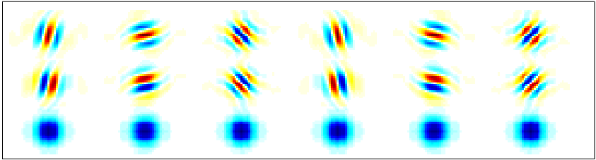
For our purposes we will make use of the overcomplete 2D wavelet basis described by [Kingsbury(2002)] and [Selesnick et al.(2006)] because of its ability to distinguish different directions (see Fig. 6). We use four wavelet scales, for a total of $4\times 64^{2}=16\,384$ wavelet and scaling coefficients $\mathbf{w}$ (four times the number of model coefficients $\mathbf{m}$). The starting point for the iterations in both the $\ell_{1}$ and $\ell_{2}$ inversions is $\mathbf{w}=\mathbf{0}$ and $\mathbf{m}=\mathbf{0}$. As explained in the previous section we renormalize the $\ell_{1}$ thresholded iteration by choosing $\alpha=\lambda_{\mathrm{max}}^{-1/2}$ (which in our case equals $4884.5$) where $\lambda_{\mathrm{max}}$ is the largest eigenvalue of $\mathbf{A}^{T}\mathbf{A}$. We let the iteration run for 1000 steps, adjust the data (two-step procedure) and let the second-step algorithm run for another 1000 steps. The threshold $\tau$ is chosen by hand in such a way as to arrive at a final value for the variance-adjusted misfit, $\chi^{2}=\|\mathbf{d}-\mathbf{A}\mathbf{m}\|_{2}^{2}\hskip 1.00006pt/\sigma^{2}$, that is approximately equal to 1848 (the number of data). The noisy data $\mathbf{d}$ are thus fit to within their standard errors $\sigma$ and no better; pushing the fit beyond this would amount to fitting the noise $\mathbf{e}$, which would lead to undesirable artifacts in the resulting model $\mathbf{m}$.

It should also be noted that the thresholding is done on pairs of wavelet coefficients: The wavelets come in pairs (at the same scale, position and orientation) that we interpret as real and imaginary part of a complex wavelet, i.e. thresholding corresponds to $(w^{\mathrm{re}}_{k},w^{\mathrm{im}}_{k})\rightarrow z=w^{\mathrm{re}}_{k}+iw^{\mathrm{im}}_{k}\rightarrow\tilde{z}=z\mathrm{S}_{\tau}(|z|)/|z|\rightarrow(\mathrm{Re}(\tilde{z}),\mathrm{Im}(\tilde{z}))$. This particular method of thresholding is borrowed from image denoising where it is found to make a big difference in avoiding artifacts [Guleryuz(2006), van Spaendonck et al.(2003), Selesnick et al.(2005)]. Furthermore, the threshold for the diagonally oriented wavelets is multiplied by $1.2395$ because $\|\nabla\psi_{\pm 45^{\circ}}\|_{1}=1.2395\|\nabla\psi_{\mathrm{other}}\|_{1}$. We choose the threshold $\tau_{\mathrm{s}}$ for the scaling coefficients to be 1/10th of the threshold $\tau_{\mathrm{w}}$ for the wavelet coefficients; since the scaling coefficients correspond to a few large-scale averages (64 in our case versus more than $16\,000$ finer-scale wavelet coefficients) it is not so important that these be sparse. Likewise, in the wavelet-basis $\ell_{2}$ inversions, we set the penalization parameter for the scaling coefficients to 1/10th the value of the penalization parameter for the wavelet coefficients.

The two-step $\ell_{1}$ algorithm takes about ten minutes for $1000+1000$ iterations on a 1.5GHz PC. The result of the $\ell_{1}$ inversion is compared with the outcome of both of the $\ell_{2}$ methods, with and without using wavelets, with the thresholding or penalization parameter $\tau$ chosen in every case to achieve the same data fit: $\chi^{2}\approx 1848$ (see Fig. 7). The number of Landweber iterations is 2000, so that the total number of two-step $\ell_{1}$ and single-step $\ell_{2}$ iterations is the same. The spatial-domain $\ell_{2}$-regularization method yields a relative modeling error $\|\mathbf{m}-\mathbf{m}^{\mathrm{input}}\|_{2}/\|\mathbf{m}^{\mathrm{input}}\|_{2}$ of about $74\%$, whereas the two-step $\ell_{1}$ method yields a relative modeling error of only $47\%$ (see Fig. 8), and is clearly less noisy (compare the middle two maps in Fig. 4). The wavelet-basis $\ell_{2}$-regularized inversion (rightmost map in Fig. 4) is only slightly less noisy, with a relative modelling error of about 55% (Fig. 8). One feature that can never be recovered in any of the reconstructions is the southern part of the rift, which does not lie between any station-event pair.

In Fig. 9 we compare the wavelet coefficients $\mathbf{w}$ of the input model, the two-step $\ell_{1}$ reconstruction and the wavelet-basis $\ell_{2}$ reconstruction. In accordance with our basic assumption, the $\ell_{1}$-regularized model is sparse in the wavelet basis. Most of the small-scale coefficients $\mathbf{w}$ are zero —in agreement with the original model on the left— indicating the effectiveness of the iterative thresholding algorithm. The wavelet coefficients of the wavelet $\ell_{2}$ reconstruction are clearly not sparse. Also this solution seems to suffer from large-scale artifacts (see Fig. 4, rightmost map).

In the leftmost plot in Fig. 10 we show $\chi^{2}$ versus $\|\mathbf{w}\|_{1}$ tradeoff curves for the $\ell_{1}$ reconstruction method, both with and without using the two-step procedure. After $1000+1000$ iterations, the $\ell_{1}$ wavelet norm $\|\mathbf{w}\|_{1}$ of the two-step reconstructed model is lower — for the same value of $\chi^{2}$ — than the corresponding norm of the model produced by 2000 iterations of the first step, with no subsequent redefinition of the data $\mathbf{d}$ and reiteration. This is an indication that 2000 total iterations is inadequate to achieve full convergence, since the fully converged model, which minimizes the functional $I_{1}(\mathbf{w})$ given in eq. (1), must be the minimum-norm model for a fixed value of $\chi^{2}$ by definition. A much larger number of iterations seems to be required to guarantee convergence. To construct the second set of tradeoff curves in Fig. 10, we employed $150\,000+150\,000$ iterations in the two-step case and $300\,000$ in the single-step case; such a large number would be prohibitive in any larger-scale, more realistic, 3D application. We have chosen to limit the iteration counts to $1000+1000$ or 2000 in all of our model-space comparisons, since any changes in the spatial-domain features of the models $\mathbf{m}$ are barely discernible to the eye with further iteration. The rightmost plot in Fig. 10 shows the principal advantage of using the two-step iteration procedure: for the same total number of iterations, either $1000+1000=2000$ or $150\,000+150\,000=300\,000$, the number of nonzero wavelet coefficients of the two-step models is always lower than the corresponding number for the single-step models. The two-step $\ell_{1}$ procedure therefore leads more quickly to a sparser wavelet-basis solution, as expected.

We also compared the single-step and two-step $\ell_{1}$ inversion methods with the corresponding $\ell_{2}$ reconstruction methods, both with and without wavelets, for a number of other input synthetic models. These include three checkerboard patterns of decreasing scale and a model similar to the geologically inspired one in Fig. 4, but with a more curvaceous low-velocity rift (see Fig. 11). Both the single-step $\ell_{1}$ reconstructions and the $\ell_{2}$ reconstructions are computed using 2000 iterations, whereas the two-step $\ell_{1}$ models are computed using $1000+1000$ iterations. In all cases, the two-step $\ell_{1}$ models are the most parsimonious and therefore to most geoscientists the most acceptable. One could consider using smoothness damping to improve the quality of the $\ell_{2}$ images; however, this would be done at the cost of resolving the sharpness of the rift structure. A nitpicker could perhaps also argue that the “rift” structure in the model produced by the $\ell_{1}$ procedure extends further northwards, albeit diminished in amplitude, whereas conventional $\ell_{2}$ regularization without wavelets exhibits a sharper cutoff, more like the input model. It achieves this sharp cutoff, however, at the expense of many artifacts elsewhere, especially along dominant ray directions. Perhaps the most noteworthy feature of the $\ell_{1}$ regularization method is its suppression of the artifacts resembling high-frequency kernel images that are streaked along surface-wave raypaths in all the $\ell_{2}$ models, to the north of the rift and within the craton. This is one of the most serious artifacts that plague conventional seismic tomography: $\ell_{2}$ regularization frequently if not always seems to enhance the well-sampled regions of the model. The $\ell_{1}$ wavelet-basis reconstructions show no signs of this familiar deficiency.

The computational bottleneck in the present 2D synthetic study is not the wavelet transform — which is fast, certainly on a model $\mathbf{m}$ of modest dimension $64\times 64$ — or even the number of iterations, but it is simply the size of the matrix $\mathbf{A}$. A significant amount of time is needed to accurately pre-compute $\mathbf{A}$, and considerable memory is needed to store the computed elements in memory; this is necessary because the product $\mathbf{A}^{T}\mathbf{A}$ is used in every step of the iteration. Doubling of the resolution in every direction results in a fourfold increase in size of the model $\mathbf{m}$, and a sixteen-fold increase in the number of elements in the square matrix $\mathbf{A}^{T}\mathbf{A}$. All calculations were performed using Matlab; software for the 2D dual-tree wavelets was downloaded from [Selesnick et al.(2006)].

We tested several new methods of regularization through wavelet decomposition of a toy 2D tomographic problem characterized by both smooth and sharp velocity anomalies. A variety of synthetic inversion experiments show that minimization of the $\ell_{1}$-norm of a wavelet decomposition of the model leads to tomographic images that are parsimonious in the sense that they use only a few wavelets and still represent both smooth and sharp features well without introducing significant blurring or artifacts. The $\ell_{1}$-norm performs significantly better than an $\ell_{2}$ regularization on either the model or its wavelet decomposition. In particular, raypath-associated artifacts are almost completely suppressed.

The choice of dual-tree complex wavelets in 2D, representing six space directions, is sufficient to avoid directional bias, and efficient in modeling both smooth features such as the cratonic structure as well as sharp features such as the rift structure in our simplified synthetic model. Numerical comparisons between the inversion results and the input model used to generate the data confirm the superiority of the $\ell_{1}$-norm regularization. Though in real-world inversions such ground-truth information is not available, one can argue that the $\ell_{1}$ inversion method serves the principle of parsimony well and is to be preferred over more common methods. If the tomographic object (such as the real earth) is too complex to be well represented by a parsimonious expansion in wavelets, neither method is able to resolve such complexity adequately with a limited data set, as shown in the bottom rows of Fig. 11, where even the $\ell_{1}$ inversions begin to show the effects of raypath distribution. In this case, we expect that the principle of parsimony can be usefully applied once a richer family of building blocks is considered.

The only drawback of the method, so far, is the slow convergence of the $\ell_{1}$ surrogate-functional iteration procedure. Our preference for the thresholded algorithm used here arises from the fact that its convergence is guaranteed even though the $\ell_{1}$ problem is nonlinear. We have introduced a two-step procedure that leads to a significant speedup; however, Fig. 10 indicates that even $1000+1000$ iterations do not suffice for complete convergence (it nevertheless produces an excellent approximation). A potentially promising approach towards further convergence improvement is to combine an efficient linear method (such as e.g. conjugate-gradient) with an adaptive thresholding scheme. This would then avoid the need to precompute the largest eigenvalue of $\mathbf{A}^{T}\mathbf{A}$ and facilitate the application of the $\ell_{1}$ method to a larger, 3D, study of body-wave tomography.

Financial support for this work was provided by NSF grant DMS-0530865. I.L. is a postdoctoral fellow with the F.W.O.-Vlaanderen (Belgium).

References

- [Candes et al.(2006)] Candes, E., Romberg, J. & Tao, T., 2006. Stable signal recovery from incomplete and inaccurate measurements, to appear in Comm. Pure Appl. Math.
- [Constable et al.(1987)] Constable, S.C., Parker, R.L. & Constable, C.G., 1987. Occam’s inversion: a practical algorithm for generating smooth models from electromagnetic sounding data, Geophys., 52, 289–300.
- [Daubechies(1992)] Daubechies, I., 1992. Ten Lectures on Wavelets, SIAM Press, Philadelphia.
- [Daubechies et al.(2004)] Daubechies, I., Defrise, M. & De Mol, C., 2004. An iterative thresholding algorithm for linear inverse problems with a sparsity constraint. Comm. Pure App. Math., 57, 1413–1541, arXiv/FA/0307152.
- [Deal & Nolet(1999)] Deal, M.M. & Nolet, G., 1999. Slab temperature and thickness from seismic tomography 2. Izu-Bonin, Japan and Kuril subduction zones, J. Geophys. Res., 104, 28803–28812.
- [Deal et al.(1999)] Deal, M.M., Nolet, G. & van der Hilst, R.D., 1999. Slab temperature and thickness from seismic tomography, 1. Method and application to Tonga, J. Geophys. Res., 104, 28789–28802.
- [de Hoop & van der Hilst(2005)] de Hoop, M. V. & van der Hilst, R. D., 2005. On sensitivity kernels for wave equation tomography, Geophys. J. Int., 160, 621–633.
- [Donoho(2004)] Donoho, D. L., 2006. For most large underdetermined systems of linear equations the minimal -norm solution is also the sparsest solution, Comm. Pure Appl. Math., 59, 797–829.
- [Dziewonski et al.(1975)] Dziewonski, A.M., Hager, B.H. & O’Connell, R.J., 1975. Large scale heterogeneities in the lower mantle, J. Geophys. Res., 82, 239–255.
- [Dziewonski & Woodhouse(1987)] Dziewonski, A.M. & Woodhouse, J.H., 1987. Global images of the Earth interior, Science, 236, 37–48.
- [Guleryuz(2006)] Guleryuz, O.G, 2003. Weighted overcomplete denoising, In Conference Record of the Thirty-Seventh Asilomar Conference on Signals, Systems and Computers, 2, 1992–1996.
- [Kingsbury(1999)] Kingsbury, N., 1999. Image processing with complex wavelets, Phil. Trans. Roy. Soc. Lond., A357, 2543–2560.
- [Kingsbury(2002)] Kingsbury, N. G., 2002. Complex wavelets for shift invariant analysis and filtering of signals, Applied and Computational Harmonic Analysis, 10, 234–253.
- [Landweber(1951)] Landweber, L., 1951. An iterative formula for Fredholm integral equations of the first kind, Am. J. Math., 73, 615–624
- [Masters et al.(1996)] Masters, G., Johnson, S., Laske, G. & Bolton, H., 1996. A shear veolcity model of the mantle, Phil. Trans. Roy. Soc. Lond., A354, 1385–1410.
- [Nolet(1987)] Nolet, G., 1987. Seismic wave propagation and seismic tomography, In G. Nolet, editor, Seismic Tomography, pages 1–23, Dordrecht, Reidel.
- [Owens et al.(1995)] Owens, T.J., Nyblade, A.A. & Langston, C.A., 1995. The Tanzania broadband experiment, IRIS Newsletter, 14, 1.
- [Portniaguine & Zhdanov(1999)] Portniaguine, O. & Zhdanov, M.S., 1999. Focusing geophysical inversion images, Geophys., 64, 874–887.
- [Selesnick et al.(2005)] Selesnick, I. W., Baraniuk, R. G. & Kingsbury, N., 2005. The dual-tree complex wavelet transform — A coherent framework for multiscale signal and image processing, IEEE Signal Processing Magazine, 22, 123-151.
- [Selesnick et al.(2006)] Selesnick, I., Cai, S. & Li, K., 2006. MATLAB implementation of wavelet transforms, http://taco.poly.edu/WaveletSoftware/.
- [Spakman & Nolet(1988)] Spakman, W. & Nolet, G., 1988. Imaging algorithms, accuracy and resolution in delay-time tomography, in N.J. Vlaar et al., editor, Mathematical Geophysics, pages 155–187, Hingham, Mass., Reidel.
- [Trampert & Snieder(1996)] Trampert, J. & Snieder, R., 1996. Model estimations biased by truncated expansions: possible artifacts in seismic tomography, Science, 271, 1257–1260.
- [VanDecar & Snieder(1994)] VanDecar, J.C. & Snieder, R., 1994. Obtaining smooth solutions to large, linear, inverse problems, Geophysics, 59, 818–829.
- [van Spaendonck et al.(2003)] van Spaendonck, R., Blu, T., Baraniuk, R. & Vetterli, M., 2003. Orthogonal Hilbert transform filter banks and wavelets, IEEE International Conference on Acoustics, Speech, and Signal Processing (ICASSP), 6, 505-508.
- [Zhou et al.(2004)] Zhou, Y., Dahlen, F.A. & Nolet, G., 2004. Three-dimensional sensitivity kernels for surface wave observables, Geophys. J. Int., 158, 142–168.
Appendix A Two-dimensional sensitivity kernels
The toy linear inverse problem used in this paper is designed to incorporate all the important characteristics of a real-world regional tomographic inversion, while at the same time being small enough to allow for repeated experimenting with reasonable CPU times on a single workstation. For this reason, we limit attention to surface-wave dispersion data, specifically perturbations in the wavenumber , presumed to be measured in rad/m, of the fundamental () Rayleigh mode at temporal frequency , measured in Hz. Finite-frequency theory based upon the Born approximation [Zhou et al.(2004)] gives a linear relationship between such wavenumber perturbations and the 3D perturbations in the fractional shear-wave velocity within the earth: