Risk Minimization through Portfolio Replication
Abstract
We use a replica approach to deal with portfolio optimization problems. A given risk measure is minimized using empirical estimates of asset values correlations. We study the phase transition which happens when the time series is too short with respect to the size of the portfolio. We also study the noise sensitivity of portfolio allocation when this transition is approached. We consider explicitely the cases where the absolute deviation and the conditional value-at-risk are chosen as a risk measure. We show how the replica method can study a wide range of risk measures, and deal with various types of time series correlations, including realistic ones with volatility clustering.
I Introduction
The portfolio optimization problem dates back to the pioneering work of Markowitz marko and is one of the main issues of risk management. Given that the input data of any risk measure ultimately come from empirical observations of the market, the problem is directly related to the presence of noise in financial time series. In a more abstract (model-based) approach, one uses Monte Carlo simulations to get “in-sample” evaluations of the objective risk function. In both cases the issue is how to take advantage of the time series of the returns on the assets in order to properly estimate the risk associated with our portfolio. This eventually results in the choice of the risk measure, and a long debate in the recent years has drawn the attention on two important and distinct clues: the mathematical property of coherence artzner99, and the noise sensitivity of the optimal portfolio. The rational behind the first of these issues lies in the need of a formal (axiomatic) translation of the basic common principles of risk management, like the fact that portfolio diversification should always lead to risk reduction. Moreover, requiring a risk measure to be coherent implies the existence of a unique optimal portfolio and a well-defined variational principle, of obvious relevance in practical cases. The second issue is also a very delicate one. In a realistic experimental set-up, the number of assets included in a portfolio can be of order to , while the length of a trustable time series hardly goes beyond a few years, i.e. . A good estimate of any extensive observable would require the condition to hold, but this is rarely the case. Instead, the ratio of assets to data points, , will be considered as a finite number.
In this note we address analytically the risk minimization problem by studying the dependence of the optimal portfolio on the ratio and on other potential external parameters. We first assume that the real distribution of returns is multinormal in order to keep the problem tactable from the analytical point of view. Generalizations to more realistic returns distributions are also presented. Our approch consists in writing down the empirical estimate of the risk measure and then reformulating the problem from the point of view of the statistical physics. We work out the analytical solution by means of the replica method mepavi and thus get some insights on the optimal portfolios. The analytical solution confirms previous results on the existence of a phase transition kondor05. The ratio plays the role of a control parameter. When it increases, there exists a sharply defined threshold value where the estimation error of the optimal portfolio diverges. A first account of our method, limited to the Expected Shortfall risk measure, has appeared in ref. es_replicas. Here we give a more general presentation, studying other risk measures and more realistic distributions of returns.
The paper is organized as follows. In section II we introduce the notations we will use throughout the paper and we formulate the problem in its general mathematical form. In section III we consider the case of the absolute deviation (AD) MAD. We present the replica calculation of the optimal portfolio and compute explicitely a noise sensitivity measure introduced in ref. pafka02. In section IV we deal with portfolio optimization under Expected Shortfall artzner99; acerbi02, which was shown to have a non-trivial phase diagram kondor05 and then studied analytically es_replicas. The striking point is that, for some values of the external parameters of the problem, the minimization problem is not well defined and thus cannot admit a finite solution. We investigate here the same feature while considering realistic distribution of returns, so as to take into account volatility clustering. The replica approch then turns into a semi-analytic and extremely versatile technique. We discuss this point and then summarize our results in section V.
II The general setting
We denote our portfolio by , where is the position on asset . We do not impose any restriction to short selling: is a real number. The global constraint induced by the total budget reads , where, due to a later mathematical convenience, we have chosen a slightly different normalization with respect to the previous literature. Calling the return of the asset and assuming the existence of a well-defined probability density function (pdf) , one is interested in computing the pdf of the loss associated to a given portfolio, i.e.
| (1) |
The complete knowledge of this pdf would lead to the precise, though still probabilistic, evaluation of the loss, thus allowing for a straightforward optimization over the space of legal portfolios. This is actually a pretty difficult task and one usually restricts to some characteristic of this pdf (e.g. its first moments, its tail beahvior), so as to capture the consequences of extremely bad events in the global loss. The actual p is not known in general, and integrals like the one in (1) are usually estimated by time series, coming from market oservations or synthetically produced by numerical simulations. Whatever the chosen risk measure then, one typically faces cost functions (to be optimized over all possible portfolios) like
| (2) |
where is the whole time series of the return and where we denoted by other possible external parameters of the risk measure. The best known example of risk measure is of course the variance, as first suggested by Markowitz. In that case the risk function is obtained by taking in (2). The evaluation of the variance implies an empirical evaluation of the covariance matrix of the underlying stochastic process, and the extremely noisy character of any estimation of has been underlined a few years ago laloux99; plerou99. However, recent studies pafka02; pafka03 have shown that the effect of the noise on the actual portfolio risk is not as dramatic as one might have expected. More in detail, a direct measure of this effect was introduced and explicitely computed in the simplest case of . In the next section, we compute the same quantity as far as the absolute deviation of the loss is concerned.
In the statistical physics approach, one studies the limit , while is finite. One introduces the partition function at inverse temperature :
| (3) |
from which any observable will be computed. For instance, the optimal cost (i.e. the minimum of the risk function in (2)) is computed from
| (4) |
It turns out that this expression depends on the actual sample (the time series ) used to estimate the risk measure. We are mainly interested in the average over all possible time series of this quantity, which we assume to be narrowly distributed around its mean value. Taking the average of eq. (4) means that we have to average the logarithm of the partition function according to the pdf . The so-called replica method allows to simplifiy this task as follows. We compute for integer and assume we can analytically continue this result to real : then . This is the strategy that we are going to use in the next sections and that will allow to compute the optimal portfolio.
III Replica analysis: Absolute Deviation
The absolute deviation measure AD is obtained by choosing in (2). No other external parameters are present here. We assume a factorized distribution
| (5) |
where the volatilities are distributed according to a pdf which we do not specify for the moment. Following the replica method, we introduce identical replicas of our portfolio and compute the average of :
where we have introduced the overlap matrix
| (7) |
as well as its conjugate , the Lagrange multipliers introduced to enforce (7). In the limit , finite, the integral in () can be solved by a saddle point method. Due to the symmetry of the integrand by permutation of replica indices, there exists a replica-symmetric saddle point mepavi: , for , and the same for . We expect the saddle point to be correct in view of the fact that the problem is linear. Under this hypothesis, which will be only justified a posteriori by a direct comparison to numerical data, the replicated partition function in () gets simplified into
| (8) | |||||
where and is the number of replicas (which will eventually go to zero). We now assume that in the low temperature limit the overlap fluctuations are of order and introduce . One can show that if stays finite at low temperatures
| (9) |
For the sake of clarity, we focus on the simple case . In the limit, the saddle point equations for (8) are
| (10) | |||||
| (11) |
where . The minimum cost function, i.e. the average of eq. (4), is found to be . Notice that (10) only admits a solution for . There is no solution to the minimization problem if the ratio of assets to data points, , is smaller than 1. On the other hand, once this condition is fulfilled, the equation (11) gives a finite at any . The asymptotic behaviour of can be worked out analytically: we introduce and consider the limit . This leads to
| (12) |
The full solution and a comparison with numerics are shown in Fig. 1 (left).


We now address the issue of noise sensitivity, for which a measure was introduced in pafka02. The idea is the following: Assume you know the true pdf of the loss (1) and you get some optimal by minimizing the absolute deviation of . We want to compare the optimal risk associated to with the one obtained by optimizing (2), i.e. the empirical estimation of the same risk measure. A fair comparison is then , with
| (13) |
where the refer to the portfolio obtained by minimizing (2). This is the quantity which we have computed by the replica approach. In our calculation we have assumed to deal with a factorized Gaussian distribution of returns (extensions to more realistic cases will be presented in the next section) and it is straightforward to prove that in this case . This corresponds in our language to , which diverges like as . Corrections to this leading behavior (which is instead the full shape of in the variance minimization problem) are needed in order to reproduce the data (right panel of Fig. 1). The comparison with the Markowitz optimal portfolio (variance minimization) indicates that the AD measure is actually less stable to perturbations: A geometric interpretation of this result can be found in ref. kondor05. Beside this fact, the interesting result is then the existence of a well defined threshold value at which the estimation error becomes infinite. This is due to the divergence of the variance of the optimal portfolio in the regime , where any minimization attempt is thus totally meaningless.
IV Expected shortfall
IV.1 The minimization problem
For a fixed value of ( in the interesting cases) the expected-shortfall (ES) of a portfolio is obtained by choosing VaR in (2), where VaR stands here for the Value-at-Risk gloriamundi. In practice, it is computed from the minimization of a properly chosen objective function rockafellar00:
| (14) |
where . Optimizing the ES risk measure over all the possible portfolios satisfying the budget constraint is equivalent to the following linear programming problem:
- •
Cost function: ;
- •
Variables: ;
- •
Constraints: .
In a previous work es_replicas we solved the problem in the case where the historical series of returns is drawn from the oversimplified probability distribution (5), with . Here we do a first step towards dealing with more realistic data and assume that the series of returns can be obtained by a sequence of normal distributions whose variances depend on time:
| (15) |
for some long range correlator which takes into account volatility correlations, and equal e.g. to a lognormal distribution.
IV.2 The replica solution
A straightforward generalization of the replica calculation presented in ref. es_replicas (and sketched in the previous section for a similar problem) allows to compute the average optimal cost for a given volatility sequence , in the limit when and stays finite. This is given by
| (16) | |||||
| (17) |
where and the function is equal to if , to is , and otherwise. The minimization over implies that
| (18) |
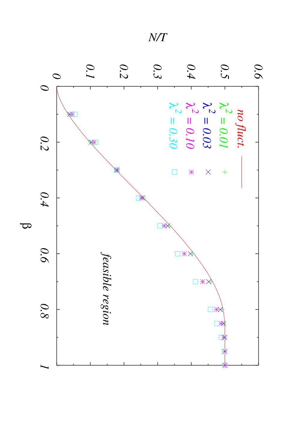
As discussed in es_replicas, the problem admits a finite solution if (17) is minimized by a finite value of . The feasible region is then defined by the condition , where and satisfy (18). This theoretical setup suggests the following semi-analytic protocol for determining the phase diagram of realistic portfolio optimization problems.
- 1.
Fix a value of , and take equal to the portfolio size you are interested in.
- 2.
- 3.
Plot vs. and find the value where this function changes its sign.
By repeating this procedure for several values of we get the phase separation line vs. .
IV.3 Results
A simple way of generating realistic volatility series consists in looking at the return time series as a cascade process mandelbrot74. In a multifractal model recently introduced muzy00 the volatility covariance decreases logarithmically: this is achieved by letting , where are Gaussian variables and
| (19) |
quantifying volatility fluctuations (the so-called ‘vol of the vol’), and being a large cutoff. A few samples generated according to this procedure are shown in Fig. 2.

The phase diagram obtained for different values of is shown in Fig. 3. A comparison with the phase diagram computed in absence of volatility fluctuations shows that, while the precise shape of the separating curve depend on the fine details of the volatility pdf, the main message has not changed: There exists a regime, , where the small number of data with respect to the portfolio size makes the optimization problem ill-defined. In the “max-loss” limit , where the single worst loss contributes to the risk measure, the threshold value does not seem to depend on the volatility fluctuations. As gets smaller than , though, the presence of these fluctuations is such that the feasible regione becomes smaller than the ideal multinormal case.
V Conclusions
In this paper we have discussed the replica approach to portfolio optimization. The rather general formulation of the problem allows to deal with several risk measures. We have shown here the examples of absolute deviation, expected shortfall and max-loss (which is simply taken as the limit case of ES). In all cases we find that the optimization problem, when the risk measure is estimated by using time series, does not admit a feasible solution if the ratio of assets to data points is larger than a threshold value. As discussed in ref. kondor05, this is a common feature of various risk measures: the estimation error on the optimal portfolio, originating from in-sample evaluations, diverges as a critical value is approached. In the expected shortfall case, we have also discussed a semi-analytic approach which is suitable for describing realistic time series. Our results suggest that, as far as volatility clustering is taken into account, the phase transition is still there, the only effect being the reduction of the feasible region. As a general remark, we have shown that the replica method may prove extremely useful in dealing with optimization problems in risk management.
Acknowledgments. We thank I. Kondor and J.-P. Bouchaud for interesting discussions. S. C. is supported by EC through the network MTR 2002-00319, STIPCO.
References
- (1) H. Markowitz, Portfolio selection: Efficient diversification of investments, J. Wiley & Sons, New York (1959).
- (2) P. Artzner, F. Delbaen, J. M. Eber, and D. Heath, Mathematical Finance 9, 203–228 (1999).
- (3) M. Mézard, G. Parisi, and M. .A. Virasoro, “Spin Glass theory and Beyond”, World Scientific Lecture Notes in Physics Vol. 9, Singapore (1987).
- (4) I. Kondor, Lectures given at the Summer School on “Risk Measurement and Control”, Rome, June 9-17, 2005; I. Kondor, S. Pafka, and G. Nagy, Noise sensitivity of portfolio selection under various risk measures, submitted to Journal of Banking and Finance.
- (5) S. Ciliberti, I. Kondor, and M. Mézard, arXiv:physics/0606015.
- (6) H. Konno, H. Yamazaki, Management Science 37, 519 (1991); H. Konno, T. Koshizuka, IIE Transactions 37, (10) 893 (2005).
- (7) C. Acerbi, and D. Tasche, Journal of Banking and Finance 26, 1487–1503 (2002).
- (8) L. Laloux, P. Cizeau, J.-P. Bouchaud, and M. Potters, Phys. Rev. Lett. 83, 1467 (1999).
- (9) V. Plerou, P. Gopikrishnan, B. Rosenow, L. Nunes Amaral, and H. Stanley, Phys. Rev. Lett. 83, 1471 (1999).
- (10) S. Pafka, and I. Kondor, Europ. Phys. J. B27, 277 (2002).
- (11) S. Pafka, and I. Kondor, Physica A319, 487 (2003).
- (12) W. H. Press, S. H. Teukolsky, W. T. Wetterling, and B. P. Flannery, “Numerical Recipes in C”, Cambridge University Press (Cambridge, UK, 1992).
- (13) see http://www.gloriamundi.org for a complete source of references.
- (14) R. Rockafellar, and S. Uryasev, The Journal of Risk 2, 21–41 (2000).
- (15) B. B. Mandelbrot, J. Fluid Mech. 62, 331 (1974).
- (16) J.-F. Muzy, J. Delour, and E. Bacry, Eur. Phys. J. B17, 537 (2000).