Capacity formulas in MWPC: some critical reflexions.
Abstract
An approximate analytical expression for ”capacitance” of MWPC configurations circulates in the literature since decades and is copied over and over again. In this paper we will try to show that this formula corresponds to a physical quantity that is different from what it is usually thought to stand for.
1 Introduction
Simple as it may seem, the concept of capacitance is a many-faced item when working in a setup with many electrodes such as it is the case in a MWPC, and it is easy to get lost. We will first analyze exactly what are the different accepted definitions of capacitance and how they are related to physical quantities that affect the functioning of the detector. Next we compare that to the established formula we will analyze here. It is the expression for ”the capacitance per unit length of each wire” in the case of a parallel wire grid, symmetrically placed between two conducting planes:
| (1) |
In this expression, is the spacing of the wires in the grid, is the distance between the wire plane and each of the conducting planes and is the radius of the wires. The formula is based upon an approximation which is excellent when is of the order of or smaller than . This equation can be found in [2] and in about all courses on gas detectors. It finds its origin in a formula in an old paper by Erskine [3], where Erskine calculated the accumulated charge on a wire plane between two planar conductors. The problem is that stated this way, the formula seems to imply that the above quantity called is, for instance, the capacitance as seen by the input of an amplifier that is connected to a single wire. This is the capacitance that will then determine the noise current induced by the equivalent voltage noise (series noise) of the amplifier. We will show in this paper that that is not true: is not that quantity. But one can already see that there is something disturbing about the given formula: namely the fact that the capacitance per wire increases when, all other dimensions equal, the wire spacing increases. Is equation 1 wrong then ? The answer is no. The formula does describe a quantity that can be called a capacitance, but it is not the usual definition — and it is not what the amplifier will see at its entrance.
2 Definitions of capacitance.
In order to understand the different possible definitions of capacitance and the confusion it can lead to, a short, elementary review is due. One cannot do better than to return to Jackson [1] in order to have a clear definition of what is ”capacitance”. There, on p. 43, it is clearly stated: ”For a system of conductors, each with potential and total charge in otherwise empty space, the electrostatic potential energy can be expressed in terms of the potentials alone and certain geometrical quantities called coefficients of capacity.”, and further:
| (2) |
We could even add to this that ”empty space” can be a confined volume with an enclosing conducting wall at ground potential. Next, Jackson writes: ”The coefficients are called capacitances while the are called the coefficients of induction.” and ”The capacitance of a conductor is therefore the total charge on the conductor when it is maintained at unit potential, all other conductors being held at zero potential.”. Note that capacitance is normally a positive quantity, while the coefficient of induction is normally a negative quantity. The coefficient of induction is the ”crosstalk” capacitance which induces charges on conductor 1 when voltages (with respect to ground) appear on conductor 2, all other conductors, including conductor 1, remaining at the same potential (with respect to ground).
It is the capacitance, as defined by Jackson, that is ”seen” by the input of an amplifier (and hence enters into the noise calculations), when all conductors are connected to (low-impedance) charge amplifiers.
Jackson also defines: ”the capacitance of two conductors carrying equal and opposite charges in the presence of other grounded conductors is defined as the ratio of the charge on one conductor to the potential difference between them”. This can then easily be worked out to result in the following expression:
| (3) |
which reduces, in the symmetrical case (, ), to:
| (4) |
This is the capacitance that is measured by a floating capacitance meter between conductors 1 and 2 (when all other conductors are put to ground potential). Note that numerically, is bigger than , because it includes also the indirect capacitive coupling in series: node 1 - ground - node 2. For instance, if there is no direct coupling () we find, indeed, that .

What is the relationship between these quantities and a network of ”equivalent capacitors” linking all conductors (nodes) amongst them and to ground, as shown in figure 1 ? Let us note by the equivalent capacitor linking nodes and , and by the equivalent capacitor linking node to ground. We now have a passive linear network to which we can apply the well-known method of node potentials [4] to write (with the Laplace variable):
| (5) |
Bringing to the other side, we obtain, on the right hand side, elements of the form which, in the time domain, come down to integrating the current over time, so can be replaced by the charge etc… and we recognize the equivalences between the capacitance matrix of Jackson and the elements of the node voltage conductance matrix above: and .
3 The meaning of Erskin’s formula
Equation 1 is based upon an expression Erskin derives in [3], when he calculates an approximate expression for the charge on each wire when wires are brought to a potential . Formula 1 is then nothing else but the ratio of . Let us consider an arbitrary wire number 1 ; using equation 2, we can then easily derive that and this is equal to : it is the capacitor element from the wire to ground in the equivalent network. But note that this is NOT the capacitance of the wire with respect to ground which is .
Unfortunately, the only way to measure, in a direct way, , is by connecting all other wires to the output of a 1:1 buffer amplifier which has a high impedance and whose input is connected to wire number 1, using all other wires in an active shielding configuration. If we then measure, with a capacitance meter, the capacitance of wire 1 w.r.t. ground, we will find . Indeed, the only capacitor on which the charge can flow is on : all capacitors are, through the servo mechanism of the buffer amplifier, kept on the same potential on both sides and do not take in any charge. This also explains the counterintuitive behavior of equation 1, that when the wires get closer, diminishes: indeed, there is more and more active shielding of the ground plane by the nearby wires, and less and less direct coupling to the ground plane, so the closer the active shielding wires come, the less capacity is measured.
However, it is now also clear that this ”capacitance” is almost never the physical quantity we need in an actual application (such as the load to the entrance of an amplifier). Only in the limit of large , when goes to 0, would become equal to , but there the approximation used is not valid anymore !
If we connect the other wires to a high-impedance (voltage) amplifier (essentially leaving them floating) this comes down to having no possibility of having a flow of net charge on these wires when wire 1 is brought from 0 to 1 V. In this case, it is as if these wires are absent, and the capacitance measured on wire 1 will be the capacitance of a single wire (limit ), which is represented by the line w1 in figure 2. As such, we should have a capacitance which is independent of ; again not the value given by . In fact, it is impossible without using active components to make the value of the capacitance as seen by an amplifier descend below the value of w1. Any passive load on the other wires will the capacitance seen by the amplifier, through , and not decrease it, as does formula 1.
We can compare the result of an exact calculation of the capacitance of wires of 1 m length (in a semi-analytic way, in a very similar way as done by Erskine [3]) of the middle wire of a set of 1, 3 or 7 wires (curves w1, w3 and w7) with equation 1. We also include a calculation of the capacitance of a single wire over a ground plane. We take the case of wires with a diameter of 20 , a distance between the wire plane and each of the ground planes of 2mm and we plot the quantities as a function of the wire spacing. We also show the values of and of for comparison.
This is shown in figure 2
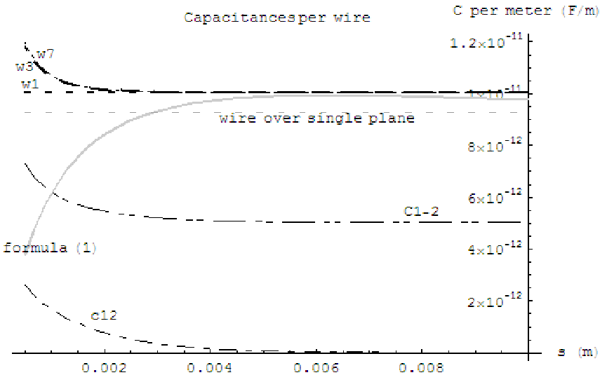
Clearly, although in a certain range, by coincidence, the numerical values of both calculations are of the same magnitude (and of the order of ), both curves have nothing to do with one another. The value needed in most applications is not the one given by formula 1.
4 Discussion
In this paper we reviewed the different aspects of the concept of ”capacitance” and used this to confront it to the calculation of a ”standard formula” for a ”capacitance” , equation 1, well-known in the world of gas detectors. From this comparison, it turns out that this quantity has a meaning, namely a capacitor value in the equivalent circuit describing the capacitive interactions between the wires and the ground plane , but that this is not the quantity it is usually claimed it is supposed to be (namely the capacitance of a single wire ). The confusion between both quantities (which are shown to have numerically different behavior) can lead to wrong applications and wrong conclusions, for instance, concerning the noise behavior of amplifiers connected to the wires of a MWPC.
References
- [1] J.D. Jackson, Classical Electrodynamics, 3rd edition, ©1999 John David Jackson, John Wiley and Sons.
- [2] F. Sauli, Principles of Operation of Multiwire Proportional and Drift Chambers, CERN 77-09, 1977.
- [3] Erskine, Nucl. Instr. Meth. 105 (1972) 565
- [4] Nahvi and Edminister, Schaum’s outlines of Electric Circuits ©2003 McGraw-Hill Companies