The remapped particle-mesh semi-Lagrangian advection scheme
Abstract
We describe the remapped particle-mesh method, a new mass-conserving method for solving the density equation which is suitable for combining with semi-Lagrangian methods for compressible flow applied to numerical weather prediction. In addition to the conservation property, the remapped particle-mesh method is computationally efficient and at least as accurate as current semi-Lagrangian methods based on cubic interpolation. We provide results of tests of the method in the plane, results from incorporating the advection method into a semi-Lagrangian method for the rotating shallow-water equations in planar geometry, and results from extending the method to the surface of a sphere.
keywords
Semi-Lagrangian advection \kspMass conservation \kspParticle-mesh method \kspSpline interpolation19991282006yy.n
C. J. Cotter and J. Frank and S. ReichThe remapped particle-mesh advection scheme
Introduction
The semi-implicit semi-Lagrangian (SISL) method, as originally introduced by Robert [16], has become very popular in numerical weather prediction (NWP). The semi-Lagrangian aspect of SISL schemes allows for a relatively accurate treatment of advection while at the same time avoiding step size restrictions of explicit Eulerian methods. The standard semi-Lagrangian algorithm (see, e.g., [19]) calculates departure points, i.e., the positions of Lagrangian particles which will be advected onto the grid during the time step. The momentum and density equations are then solved along the trajectory of the particles. This calculation requires interpolation to obtain velocity and density values at the departure point. It has been found that cubic interpolation is both accurate and computationally tractable (see, e.g., [19]).
Ideally, as well as being efficient and accurate, a density advection scheme should exactly preserve mass in order to be useful for, e.g., climate prediction or atmospheric chemistry calculations. Recent developments have involved computing the change in volume elements, defined between departure and arrival points, making use of a technique called cascade interpolation [14]. Several such methods have been suggested in recent years, including the methods of Nair et al [11, 12, 13] and the SLICE schemes of Zerroukat et al [23, 24, 26, 25].
In this paper we give a new density advection scheme, the remapped particle-mesh method, which is based on the particle-mesh discretisation for the density equation used in the Hamiltonian Particle-Mesh (HPM) method suggested by Gottwald, Frank & Reich [3], which itself was a combination of smoothed particle-hydrodynamics [7, 5] and particle-in-cell methods [6]. The particle-mesh method provides a very simple discretisation which conserves mass by construction, and may be adapted to nonplanar geometries such as the sphere [4]. In this paper we show that an efficient scheme can be obtained by mapping the particles back to the grid after each time step. Our numerical results show that this scheme is at least as accurate as standard semi-Lagrangian advection using cubic interpolation at departure points. We show how the method may be included in the staggered semi-Lagrangian schemes, proposed by Staniforth et al [20] and Reich [15], and show how to adapt it to spherical geometry.
In section The remapped particle-mesh semi-Lagrangian advection scheme we describe the particle-mesh discretisation for the density equation. The method is modified to form the remapped particle-mesh method in section The remapped particle-mesh semi-Lagrangian advection scheme. We discuss issues of efficient implementation in section The remapped particle-mesh semi-Lagrangian advection scheme. In section The remapped particle-mesh semi-Lagrangian advection scheme we give numerical results for advection tests in planar geometry and on the sphere, as well as results from rotating shallow-water simulations using the remapped particle-mesh method in the staggered leapfrog scheme [15]. We give a summary of our results and discussion in section The remapped particle-mesh semi-Lagrangian advection scheme.
Continuity equation and particle advection In this section we describe the particle-mesh discretisation for the density equation. This discretisation forms the basis for the remapped particle-mesh method discussed in this paper. For simplicity, we restrict the discussion to two-dimensional flows.
We begin with the continuity equation
| (1) |
where is the density and is the fluid velocity. We write (1) in the Lagrangian formulation as
| (2) | |||||
| (3) |
where is the density at time at a fixed Eulerian position ,
| (4) |
is the Lagrangian time derivative,
| (5) |
is a Lagrangian particle position at time with initial position , and is the initial density at .
To discretise the integral representation (3), we introduce a finite set of Lagrangian particles , , and a fixed Eulerian grid , . Then we approximate the Eulerian grid density by
| (6) |
where are basis functions, which satisfy . The initial particle positions are assumed to form a grid and is equal to the area of the associated grid cell. Equation (6) may be simplified to
| (7) |
where
| (8) |
is the “mass” of particle .
Let us now also request that the basis functions satisfy the partition-of-unity (PoU) property
| (9) |
for all . This ensures that the total mass is conserved since
| (10) |
which is constant. The time evolution of the particle positions is simply given by
| (11) |
Given a time-dependent (Eulerian) velocity field , we can discretise (8) and (11) in time with a simple differencing method:
| (12) | |||||
| (13) |
In [3], this discretisation was combined with a time stepping method for the momentum equation to form a Hamiltonian particle-mesh method for the rotating shallow-water equations. The masses were kept constant throughout the simulation. In this paper, we instead combine the discretisation with a remapping technique so that the particles trajectories start from grid points at the beginning of each time step. Our remapping approach requires the assignment of new particle “masses” in each time step and, hence, is fundamentally different from semi-Lagrangian remapping strategies described, for example, in [11].
Remapped particle-mesh method
In this section, we describe the remapped particle-mesh method for solving the continuity equation. The aim is to exploit the mass conservation property of the particle-mesh method whilst keeping an Eulerian grid data structure for velocity updates. To achieve this we reset the particles to an Eulerian grid point at the beginning of each time step, i.e.,
| (14) |
This step requires the calculation of new particle “masses” , , according to
| (15) |
for given densities . This is the remapping step. We finally step the particles forward and calculate the new density on the Eulerian grid using equations (12)-(13) with . Note that the Lagrangian trajectory calculation (12) can be replaced by any other consistent upstream approximation. Exact trajectories for a given time-independent velocity field will, for example, be used in the numerical experiments.
The whole process is mass conserving since the PoU property (9) ensures that
| (16) |
Efficient implementation
This density advection scheme can be made efficient since all the interpolation takes place on the grid; this means that the same linear system of equations, characterized by (15), is solved at each time step. The particle trajectories are uncoupled and thus may even be calculated in parallel.
The computation of the particle masses in (15) leads to the solution of a sparse matrix system. We discuss this issue in detail for (area-weighted) tensor product cubic -spline basis functions, defined by
| (17) |
where is the cubic B-spline
| (18) |
The basis functions satisfy
| (19) |
and
| (20) |
as required.
A few basic manipulations reveal that (15) becomes equivalent to
| (21) |
where
| (22) |
are the standard second-order central difference approximations, and we replaced index by , i.e., we write , , etc. from now on. Eq. (21) implies that the particle masses can be found by solving a tridiagonal system along each grid line (in each direction).
If the cubic spline in (17) is replaced by the linear spline
| (23) |
then the system (15) is solved by
| (24) |
The resulting low-order advection scheme possesses the desirable property that for all implies that for all , and so that monotonicity is also preserved.
On a more abstract level, conservative advection schemes can be derived for general (e.g. triangular) meshes with basis functions , which form a partition of unity. An appropriate quadrature formula for (3) leads then to a discrete approximation of type (7). This extension will be the subject of a forthcoming publication.
Extension to the sphere In this section we suggest a possible implementation of the remapped particle-mesh method for the density equation on the sphere. The method follows the particle-mesh discretisation given by Frank & Reich [4], combined with a remapping to the grid.
We introduce a longitude-latitude grid with equal grid spacing . The latitude grid points are offset a half-grid length from the poles. Hence we obtain grid points , where , , , , and the grid dimension is .
Let denote the (area-weighted) tensor product cubic B-spline centered at a grid point with longitude-latitude coordinates , i.e.
| (25) |
where are the spherical coordinates of a point on the sphere, is the cubic B-spline as before, and
| (26) |
We convert between Cartesian and spherical coordinates using the formulas
| (27) |
and
| (28) |
At each time step we write the fluid velocity in 3D Cartesian coordinates and step the particles forward. We then project the particle positions onto the surface of the sphere as described in [4]. The Lagrangian trajectory algorithm is then:
| (29) |
where is a Lagrange multiplier chosen so that on a sphere of radius . This alogrithm can be replaced by any other consistent approximation upstream Lagrangian trajectories. Exact trajectories are, for example, used in the numerical experiments.
We compute the particle masses by solving the system
| (30) |
for given densities . The density at time-level is then determined by
| (31) |
Note that the system (30) is equivalent to
| (32) |
and can be solved efficiently as outlined in section The remapped particle-mesh semi-Lagrangian advection scheme. The implementation of the remapping method is greatly simplified by making use of the periodicity of the spherical coordinate system in the following sense. The periodicity is trivial in the longitudinal direction. For the latitude, a great circle meridian is formed by connecting the latitude data separated by an angular distance in longitude (or grid points). See, for example, the paper by Spotz, Taylor & Swarztrauber [18]. It is then efficient to solve the system (32) using a direct solver.
Conservation of mass is encoded in
| (33) |
which holds because of the PoU property
| (34) |
Numerical results
1D convergence test Following [26], we test the convergence rate of our method for one-dimensional uniform advection of a sine wave over a periodic domain . The initial distribution is
| (35) |
and the velocity field is . The 1D version of our method is used to solve the continuity equation
| (36) |
The experimental setting is equivalent to that of [26]. Table 1 displays the convergence of errors as a function of resolution . Note that the results from Table 1 are in exact agreement with those displayed in Table I of [26] for the parabolic spline method (PSM) and fourth-order accuracy is observed.
| 8 | 16 | 32 | 64 | 128 | 256 | 512 | |
|---|---|---|---|---|---|---|---|
| 0.549E-02 | 0.254E-03 | 0.143E-4 | 0.872E-6 | 0.541E-07 | 0.337E-08 | 0.211E-09 |
Cubic Interpolation Cubic Spline


2D planar advection: Slotted-cylinder problem
Convergence is now examined for a more realistic test case. Since we use higher-order interpolation the initial density profile needs to be sufficiently smooth. On the other hand, relatively sharp gradients should be present to pose a challenge to the advection scheme. We decided to use a smoothed slotted-cylinder obtained by applying a modified Helmholtz operator to the standard sharp-edged slotted cylinder [22]. The smoothing length is set to . See panel (a) in Fig. 1.
We compare the newly proposed scheme to the standard SL advection scheme based on backward trajectories and bicubic interpolation (see, e.g. [19]). To exclude any errors from the trajectory calculation we use a double periodic domain of size and apply a constant velocity field , . The time-step is and the simulations are run over a period of time units. Note that the initial density profile returns to its original position after time units. This allows us to introduce the error
| (37) |
for .
Simulations are performed on a spatial grid with , , and . Errors (37) are provided in Fig. 2. It can be seen that the newly proposed method is more accurate than the standard SL advection scheme and that the newly proposed method achieves second-order accuracy as a function of spatial resolution (for fixed time-steps ). Detailed results from simulations with can be found in Fig. 1.
Following the discussion of [26] the reduced order can be explained by the fact that the Helmholtz operator leads to an approximate spectral decay in the Fourier transform of the initial density . As also explained in [26], the improved convergence of our spline-based method over the traditional bicubic SL method is to be expected.

We also implemented the standard rotating slotted-cylinder problem as, for example, defined in [10, 23]. See [23] for a detailed problem description and numerical reference solutions. Corresponding results for the newly proposed advection scheme can be found in Fig. 3.

2D planar advection: Idealized cyclogenesis problem
The idealized cyclogenesis problem (see, e.g., [10, 23]) consists of a circular vortex with a tangential velocity , where is the radial distance from the centre of the vortex and is a constant chosen such that the maximum value of is unity. The analytic solution is
| (38) |
where is the angular velocity and . The experimental setting is that of [10, 23]. In particular, the domain of integration is with a grid. The time step is and a total of 16 time steps is performed. Numerical reference solutions can be found in [23] for the standard bicubic and several conservative SL methods. The corresponding results for the newly proposed advection scheme can be found in Fig. 4.
Spherical advection: Solid body rotation
Solid body rotation is a commonly used experiment to test an advection scheme over the sphere. We apply the experimental setting of [11, 12, 13, 24]. The initial density is the cosine bell,
| (39) |
where ,
| (40) |
and . The bell is advected by a time-invariant velocity field
| (41) | |||||
| (42) |
where are the velocity components in and direction, respectively, and is the angle between the axis of solid body rotation and the polar axis of the sphere.
| 0.0492 | 0.0591 | 0.0627 | |
| 0.0336 | 0.0393 | 0.0397 | |
| 0.0280 | 0.0367 | 0.0374 |
Experiments are conducted for , , and . Analytic trajectories are used and is chosen such that 256 time steps correspond to a complete revolution around the globe (the radius of the sphere is set equal to one). Accuracy is measured as relative errors in the , , and norms (as defined, for example, in [24]). Results are reported in Table 2 for a grid (i.e., ).
Note that (32) may lead to a non-uniform distribution of particle masses near the polar cap regions for meridional Courant numbers . This can imply a loss of accuracy if a “heavy” extra-polar particle moves into a polar cap region. We verified this for 72, 36 and 18, respectively, time steps per complete revolution (implying a meridional Courant number of , , and , respectively). It was found that the accuracy is improved by applying a smoothing operator along lines of constant near the polar caps, e.g.,
| (43) |
, . Here denotes the density approximation obtained from (31). The filter (43) is mass conserving and acts similarly to hyper-viscosity. The disadvantage of this simple filter is that under zero advection.
(a) 72 time steps (b) 36 time steps (c) 18 time steps
| 0.0491 | 0.0283 | |
| 0.0468 | 0.0168 | |
| 0.0723 | 0.0122 |
2.3264 0.0222 1.5124 0.0137 1.1383 0.0151 2.3217 0.0143 1.5126 0.0105 1.0764 0.0143
Results for and , respectively, and 72, 36 and 18 time steps, respectively, are reported in Table 3. It is evident that filtering by (43) improves the results significantly. Corresponding results for standard advection schemes can be found in [11] for the case of 72 time steps per complete revolution.
Spherical advection: Smooth deformational flow
To further evaluate the accuracy of the advection scheme in spherical geometry, we consider the idealized vortex problem of Doswell [1]. The flow field is deformational and an analytic solution is available (see [9, 11] for details).
We summarize the mathematical formulation. Let be a rotated coordinate system with the north pole at with respect to the regular spherical coordinates. We consider rotations of the coordinate system with an angular velocity , i.e.,
| (44) |
where
| (45) |
An analytic solution to the continuity equation (1) in coordinates is provided by
| (46) |
| 3 | 6 | |
|---|---|---|
| 0.0019 | 0.0055 | |
| 0.0062 | 0.0172 | |
| 0.0324 | 0.0792 |
Simulations are performed using a grid and a step size of . The filter (43) is not applied. The exact solution (evaluated over the given grid) and its numerical approximation at times and are displayed in Fig. 5. The relative , and errors (as defined in [24]) can be found in Table 4. These errors are comparable to the errors reported in [11, 24] for the standard SL bicubic interpolation approach.


Rotating shallow-water equations in planar geometry
To demonstrate the behavior of the new advection scheme under a time-dependent and compressible velocity field, we consider the shallow-water equations (SWEs) on an -plane [2, 17]:
| (47) | |||||
| (48) | |||||
| (49) |
Here is the fluid depth, is the gravitational constant, and is twice the (constant) angular velocity of the reference plane.
Let denote the maximum value of over the whole fluid domain. We also introduce the fluid depth perturbation . The perturbation satisfies the continuity equation
| (50) |
which we solve numerically using the newly proposed scheme. The overall time stepping procedure is given by the semi-Lagrangian Störmer-Verlet (SLSV) method proposed by Reich [15] with only equation (5.7) from [15] being replaced by the following steps:
- (i)
- (ii)
Solve (50) over a full time step using the newly proposed scheme with velocities and initial fluid depth perturbation . Denote the resulting fluid depth by .
- (iii)
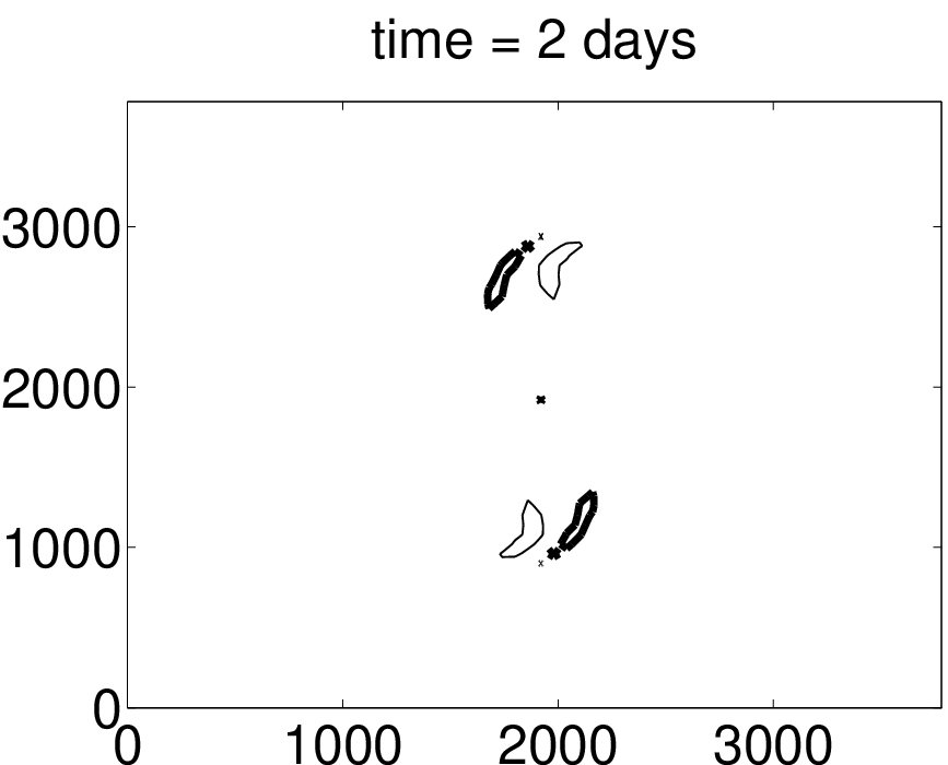
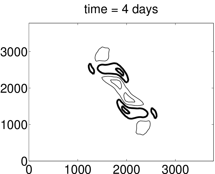
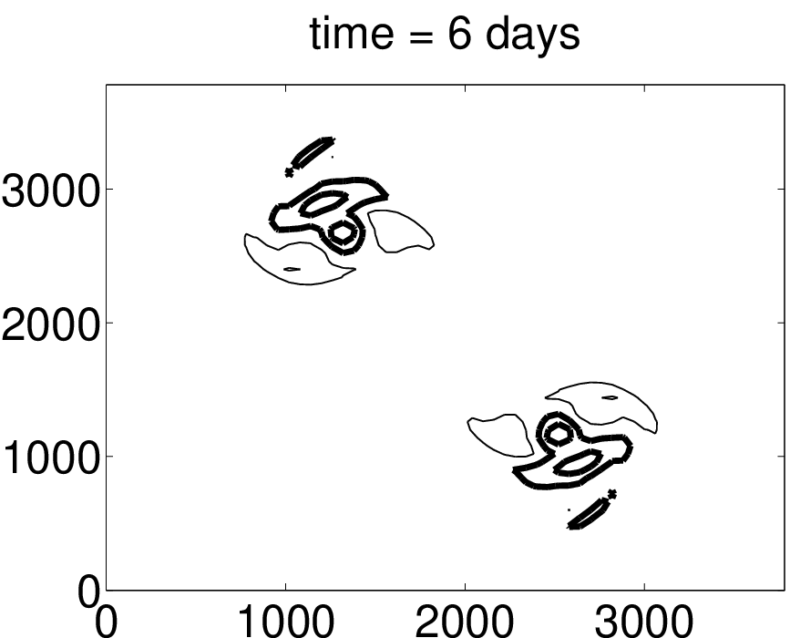
The method has been implemented using the standard C-grid [2] over a double periodic domain with 3840 km (see [20] for details). The grid size is 60 km. The time step is 20 min and the value of corresponds to an -plane at 45o latitude. The reference height of the fluid is set to 9665 m. The Rossby radius of deformation is 3000 km. Initial conditions are chosen as in [20, 15] and results are displayed in an identical format for direct comparison.
To assess the new discretization, results are compared to those from a two-time-level semi-implicit semi-Lagrangian (SISL) method with a standard bicubic interpolation approach to semi-Lagrangian advection (see, e.g., [8, 21]). It is apparent from Fig. 6 that both simulations yield similar results in terms of potential vorticity advection. Furthermore, the results displayed in Fig. 6 are nearly identical to those displayed in Fig. 6.1 of [15]. The implication is that the newly proposed advection scheme in manner very similar to the traditional SL interpolation scheme for this particular test problem. This result in not unexpected as the fluid depth remains rather smooth throughout the simulation.
SLSV SLSV-SISL




Summary and outlook
A computationally efficient and mass conserving forward trajectory semi-Lagrangian approach has been proposed for the solution of the continuity equation (1). At every time step a “mass” is assigned to each grid point which is then advected downstream to a (Lagrangian) position. The gridded density at the next time step is obtained by evaluating a bicubic spline representation with the advected masses as weights. The main computational cost is given by the need to invert tridiagonal linear systems in (21). Computationally efficient iterative or direct solvers are available. We also proposed an extension of the advection scheme to spherical geometry. A further generalization to 3D would be straightforward. Numerical experiments show that the new advection scheme achieves accuracy comparable to standard non-concerving and published conserving SL schemes.
We note that the proposed advection scheme can be used to advect momenta according to
| (51) |
This possibility is particularly attractive in the context of the newly proposed semi-Lagrangian Störmer-Verlet (SLSV) scheme [15].
We would like to thank Nigel Wood for discussions and comments on earlier drafts of this manuscript.
References
- [1] C.A. Doswell. A kinematic analysis of frontogenesis associated with a nondivergent vortex. J. Atmos. Sci., 41:1242–1248, 1984.
- [2] D.R. Durran. Numerical Methods for Wave Equations in Geophysical Fluid Dynamics. Springer-Verlag, Berlin Heidelberg, 1998.
- [3] J. Frank, G. Gottwald, and S. Reich. The Hamiltonian particle-mesh method. In M. Griebel and M.A. Schweitzer, editors, Meshfree Methods for Partial Differential Equations, volume 26 of Lect. Notes Comput. Sci. Eng., pages 131–142, Berlin Heidelberg, 2002. Springer-Verlag.
- [4] J. Frank and S. Reich. The Hamiltonian particle-mesh method for the spherical shallow water equations. Atmos. Sci. Lett., 5:89–95, 2004.
- [5] R.A. Gingold and J.J. Monaghan. Smoothed Particle Hydrodynamics: Theory and application to non-spherical stars. Mon. Not. R. Astr. Soc., 181:375–389, 1977.
- [6] F. Harlow. The particle-in-cell computing methods for fluid dynamics. Methods Comput. Phys., 3:319–343, 1964.
- [7] L.B. Lucy. A numerical approach to the testing of the fission hypothesis. Astron. J., 82:1013–1024, 1977.
- [8] A. McDonald and J.R. Bates. Improving the estimate of the departure point in a two-time level semi-Lagrangian and semi-implicit scheme. Mon. Wea. Rev., 115:737–739, 1987.
- [9] R.D. Nair, J. Coté, and A. Staniforth. Cascade interpolation for semi-Lagrangian advection over the sphere. Q.J.R. Meteor. Soc., 125:1445–1468, 1999.
- [10] R.D. Nair, J. Coté, and A. Staniforth. Monotonic cascade interpolation for semi-Lagrangian advection. Q.J.R. Meteor. Soc., 125:197–212, 1999.
- [11] R.D. Nair and B. Machenhauer. The mass-conservative cell-integrated semi-Lagrangian advection scheme on the sphere. Mon. Wea. Rev., 130:649–667, 2002.
- [12] R.D. Nair, J.S. Scroggs, and F.H.M. Semazzi. Efficient conservative global transport schemes for climate and atmospheric chemistry models. Mon. Wea. Rev., 130:2059–2073, 2002.
- [13] R.D. Nair, J.S. Scroggs, and F.H.M. Semazzi. A forward-trajectory global semi-Lagrangian transport scheme. J. Comput. Phys., 190:275–294, 2003.
- [14] R.J. Perser and L.M. Leslie. An efficient interpolation procedure for high-order three-dimensional semi-Lagrangian models. Mon. Wea. Rev., 119:2492–2498, 1991.
- [15] S. Reich. Linearly implicit time stepping methods for numerical weather prediction. BIT, in press, 2006.
- [16] A. Robert. A semi-Lagrangian and semi-implicit numerical integration scheme for the primitive meteorological equations. Jpn. Meteor. Soc., 60:319–325, 1982.
- [17] R. Salmon. Lectures on Geophysical Fluid Dynamics. Oxford University Press, Oxford, 1999.
- [18] W.F. Spotz, M.A. Taylor, and P.N. Swarztrauber. Fast shallow-water equations solvers in latitude-longitude coordinates. J. Comput. Phys., 145:432–444, 1998.
- [19] A. Staniforth and J. Coté. Semi-Lagrangian integration schemes for atmospheric models – A review. Mon. Wea. Rev., 119:2206–2223, 1991.
- [20] A. Staniforth, N. Wood, and S. Reich. A time-staggered semi-Lagrangian discretization of the rotating shallow-water equations. Q.J.R. Meteorolog. Soc., submitted, 2006.
- [21] C. Temperton and A. Staniforth. An efficient two-time-level semi-Lagrangian semi-implicit integration scheme. Q.J.R. Meteorol. Soc., 113:1025–1039, 1987.
- [22] S.T. Zalesak. Fully multidimensional flux-corrected transport algorithms for fluids. J. Comput. Phys., 31:335–362, 1979.
- [23] M. Zerroukat, N. Wood, and A. Staniforth. SLICE: A semi-Lagrangian inherently conserving and efficient scheme for transport problems. Q.J.R. Meteorol. Soc., 128:801–820, 2002.
- [24] M. Zerroukat, N. Wood, and A. Staniforth. SLICE-S: A semi-Lagrangian inherently conserving and efficient scheme for transport problems on the sphere. Q.J.R. Meteorol. Soc., 130:2649–2664, 2004.
- [25] M. Zerroukat, N. Wood, and A. Staniforth. Application of the parabolic spline method (PSM) to a multi-dimensional conservative semi-Larangian transport scheme (SLICE). Int. J. Numer. Meth. Fluids, submitted, 2006.
- [26] M. Zerroukat, N. Wood, and A. Staniforth. The parabolic spline method (PSM) for conservative transport problems. Int. J. Numer. Meth. Fluids, in press, 2006.
*