Falling of a viscous jet onto a moving surface

In the flow of a viscous fluid jet falling onto a moving surface different flow regimes can be distinguished, as is easily observed if one pours syrup onto a pancake (Figs 1 and 2). If the syrup is poured from a large height and the bottle moves slowly, then the syrup thread is perfectly vertical (Fig. 1). If the bottle is held closer to the pancake and moved relatively fast, however, then the flow of syrup becomes curved.

Note the difference in behavior at the touchdown point. In the straight case, the jet hits the surface at right angles, and a little puddle forms on the surface from which a thicker ‘jet’ is transported away by the surface movement (Fig. 1). Since the flow velocity of the surface jet equals the surface velocity, conservation of mass implies that at the touchdown point the particle velocity in the free jet is larger than the velocity of the surface. In the curved case, however, the jet does not thicken at touchdown, and the free jet meets the surface tangentially.

There is a large body of literature on viscous jets or sheets that impinge upon fixed surfaces, where one can observe folding of viscous sheets [Scorobogatiy, Ribe1], coiling of viscous jets [Ribe2], and viscous fluid buckling [Cruickshank]. The fact that in these cases the surface is stationary is essential; to our knowledge the current work is the first study of a viscous jet that falls upon a moving surface.

In Section 2, we construct a mathematical model of the flow, where we first concentrate on the curved jet of Fig. 2. We model the flow as a thin, Newtonian jet of a priori unknown length. In Section 3, the original system of equations is transformed to a first-order differential equation for the flow velocity and two additional relations for two unknown parameters. In Section 4, we show that in a certain parameter regime the original system admits a unique solution, and we give a convenient characterization of the relevant part of parameter space. In Section 5, we present the solution algorithms for the model equations. Results for various model parameters are shown in Section 6, and in Section 7, we discuss our results and give some conclusions.

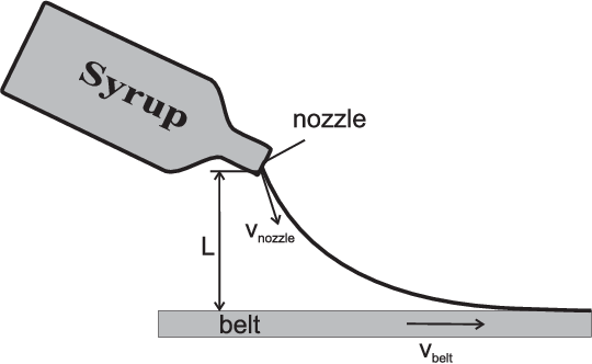
A thin stream of Newtonian fluid with viscosity $\eta$ and density $\rho$ is falling from the nozzle of a bottle onto a moving belt (Fig. 3). We use the theory of thin jets (see e.g. [Yarin]) and thus describe the jet as a curve.

The magnitude of the flow velocity at the nozzle is $v_{\mathrm{nozzle}}$, the belt velocity is $v_{\mathrm{belt}}$, and the distance between the nozzle and the belt is $L$. The flow of the fluid is stationary and the jet has a curved shape. We restrict ourselves to curves under tension and therefore require that

In Lemma 1, we show that for a curved jet the flow velocity increases from the nozzle to the belt which justifies (1).

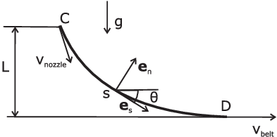
The part of the jet between the nozzle and the belt is represented by its center line, the curve $CD$ in Fig. 4. The point $C$ indicates the nozzle and the point $D$ indicates the contact with the belt. The acceleration of gravity is $\mathbf{g}$ and the belt surface is perpendicular to $\mathbf{g}$. We parameterize the center line by arclength $s$ ($s=0$ at $C$, and $s=s_{\mathrm{end}}$ at $D$). For each point on the curve we define a local orthonormal coordinate system $\mathbf{e}_{s}(s),\mathbf{e}_{n}(s)$ consisting of the tangent and normal unit vectors at the point $s$. The angle between $\mathbf{e}_{s}(s)$ and the belt surface is $\Theta(s)$. The cross-sectional area at $s$ is $\mathcal{A}(s)$, and the average velocity of the fluid at this point is $\mathbf{v}(s)=v(s)\mathbf{e}_{s}(s)$.

The flow of fluid is described by the equations of conservation of mass and balance of momentum [Yarin, (4.18)], which for stationary flow are

respectively, where by ^′ we denote differentiation with respect to $s$. The longitudinal force $P(s)$ is obtained from the constitutive law for a Newtonian viscous fluid

Here $\eta_{T}$ is the Trouton elongational viscosity, which for a Newtonian fluid equals $3\eta$ [Yarin].

Using (2) and (4), we write the balance of momentum (3) in components in the coordinate system $\mathbf{e}_{s}(s),\mathbf{e}_{n}(s)$, as

where $\mu$ is equal to three times the kinematic viscosity, i.e. $\mu=3\eta/\rho$.

Since system (5–6) is of second order with respect to the velocity $v(s)$ and of first order with respect to the angle $\Theta(s)$, we need two boundary conditions for $v(s)$ and one for $\Theta(s)$. For $v(s)$ we know the velocity of the jet at the nozzle (point $C$) and the velocity at the contact with the belt (point $D$)

Note that the length $s_{\mathrm{end}}$ of the jet $CD$ is unknown. The angle $\Theta(s)$ at the contact with the belt is zero, so

Because the length of the belt $s_{\mathrm{end}}$ is unknown in advance, we need an additional condition relating $s_{\mathrm{end}}$ to the distance $L$ between the nozzle and the belt

The equations (5) and (6) together with the three boundary conditions (7–9), and the additional condition (10) form the complete system for the unknowns $v(s)$, $\Theta(s)$ and $s_{\mathrm{end}}$.

We next make the equations dimensionless. We scale the length $s_{\mathrm{end}}$ with respect to $\mu/v_{\mathrm{belt}}$, reverse the direction of $s$, and move the origin of $s$ to the point $D$, i.e. $\tilde{s}:=v_{\mathrm{belt}}(s_{\mathrm{end}}-s)/\mu$. The velocity $v(s)$ is scaled with respect to the velocity of the belt $v_{\mathrm{belt}}$, i.e., $v_{\mathrm{belt}}\tilde{v}(\tilde{s}):=v(s)$. Also we introduce a new angle $\tilde{\Theta}(\tilde{s}):=\Theta(s)$. The scaled version of (5–10) reads

Here

All these parameters are positive and $B$ is the Reynolds number. The prime now denotes differentiation with respect to $\tilde{s}$, and in the sequel we omit the tildes.

By introducing a new variable $\xi(s)$

we can rewrite the equations (11–12) as

For the variable $\xi(s)$ it is necessary to provide an initial value. To compute it, we need to know values of $v(s)$ and $v^{\prime}(s)$ at the same point. Because we do not know a value of $v^{\prime}(s)$ at any point we prescribe a value of $\xi(s)$ at $s=0$,

Here we restrict ourselves to a negative initial value for $\xi$. Further in this section, see (33) and (34), we explain our choice of the form for the initial value for $\xi(s)$. The value $w$ is unknown in advance and is determined by the requirement that a solution of (18–20) has to satisfy the conditions (16) and (14).

Next, we replace the material coordinate $s$ by the time $t$, according to

in the system of equations (18–20) together with the conditions (13–16) and (21), and we obtain

Here

represents the dimensionless time necessary to flow from the nozzle to the belt, which is unknown in advance.

To solve the equations (22) and (23) we multiply (22) by $\sin\Theta(t)$ and (23) by $\cos\Theta(t)\xi(t)$ and add them, to obtain

We integrate (30) with respect to $t$ and use the initial condition (26) to obtain

By eliminating $\sin\Theta(t)$ from (31) and substituting it into (22) we derive the differential equation for $\xi(t)$

which has the solution

Here we have to choose a correct branch of the square root (33). The branch with the positive sign gives negative $\sin\Theta(t)$, see (31), which implies an upward-sloping jet; the physically reasonable choice is therefore the branch with the negative sign. With the initial condition (21) we get

and from (31) and (34) we find

Summarizing, the problem (22–29) simplifies to

The unknowns of the problem (36–39) are the velocity $v(t)$ and the two positive parameters $w$ and $t_{\mathrm{end}}$.

We reformulate the problem (36–39) as an algebraic equation for the parameter $w$. First we formulate properties of a solution $v(\cdot,w)$ of (36–37) for given $w\geq 0$ .

In order to solve (36)-(39) we need to find $w$ for which (38)-(39) are satisfied. Knowing a correct value of $w$, we can obtain a solution $v(t)$ which leads to a solution of the original problem (11)-(16). Therefore, next we concentrate on finding a correct $w$.

By Lemma 1, part 2 the integrable function is bounded from above and the integral converges.

In the next three lemmas we will show some properties of $I(w)$ which lead to a characterization of existence and uniqueness of a solution to (44).

Summarizing the results of previous lemmas, we formulate a theorem of existence and uniqueness of a solution to the original problem (11–16).

The theorem follows simply from Lemmas 4, 5, and 6.

In Section 5, we describe two algorithms for computing $I(0;A,v_{\mathrm{nozzle}})$ as a function of $A$ and $v_{\mathrm{nozzle}}$, resulting in the graph of Fig. 5. As a consequence of Theorem 7, a solution to the original problem (11–16) exists only if the point $(A,v_{\mathrm{nozzle}},B)$ is below the surface $I(0;A,v_{\mathrm{nozzle}})$.

Note: Non-existence of a curved-jet solution. When the condition (49) is not satisfied, then there exists no solution to the curved-jet equations (11–16). What happens to a viscous jet in this parameter range is not clear. It is possible that a stable straight jet exists ($\Theta\equiv\pi/2$); close to the transition between existence and non-existence the curved-jet solution becomes straight (see Fig. 8), supporting this possibility. Other possibilities are coiling (in three dimensions) or buckling (in two dimensions), possibly coexisting with a steady straight jet that is dynamically unstable.

At this moment the issue is open, in part since it is unclear which boundary condition at the lower end of the jet best reflects the physical situation. We plan to return to this question in a future publication.

The problem of this paper gives rise to two slightly different numerical questions. The first question arises in making a phase diagram such as Fig. 6: in order to distinguish between existence and non-existence of a curved jet we need to calculate $I(0;A,v_{\mathrm{nozzle}})$ and check the existence condition $I(0;A,v_{\mathrm{nozzle}})>B$ (49). The second question arises when this condition is fulfilled: by Corollary 3 we then need to find $w>0$ such that $I(w;A,v_{\mathrm{nozzle}})=B$, from which $v$ and $\Theta$ can then be determined by solving (36–37) and using (35).

The main differential equation (36) can be solved either analytically or numerically, giving rise to two different methods.

Method 1. When $w=0$, it is possible to solve the problem (36–37) analytically (Appendix A). The rescaled domain size $z^{*}$ is then to be determined implicitly from

where the $J_{\alpha}$ are the Bessel functions of the first kind. We then calculate $t_{\mathrm{end}}(0)$ and $I(0;A,v_{\mathrm{nozzle}})$ as

This method only is available for the special case $w=0$.

Method 2. Alternatively, one may integrate (36) numerically until the condition $v(t;0)=v_{\mathrm{nozzle}}$ is reached. The integral $I(w;A,v_{\mathrm{nozzle}})$ can be computed numerically as well. This method is available for all $w\geq 0$.

We solve (44) by the bisection method, supplemented with an upper bound on $w$ that follows from the estimate (40): since for all $w$,

we have

and therefore $At_{\mathrm{end}}(w)^{2}<2/v_{\mathrm{nozzle}}$. We thus estimate

Therefore the solution $w$ of (44) satisfies the a priori estimate

From Theorem 7 it follows that if the parameters $A$, $B$, and $v_{\mathrm{nozzle}}$ satisfy (49), then there exists a solution to the stationary curved-jet equations (5–10) (or equivalently (36–39)); otherwise the jet is vertical, or a stationary solution does not exist.

Fig. 6 shows the region of existence of such a curved-jet solution.

As a reference configuration for the numerical experiments shown below we consider syrup with viscosity $\eta=3.2\,\mathrm{Pa\,s}$ and density $\rho=1000\,\mathrm{kg/m^{3}}$ pouring from the height $L=2\cdot 10^{-2}\,\mathrm{m}$. The velocities of the belt and the flow at the nozzle are $v_{\mathrm{belt}}=0.5\,\mathrm{m/s}$ and $v_{\mathrm{nozzle}}=0.05\,\mathrm{m/s}$, respectively.

Fig. 7 shows curves in non-dimensional parameter space $(A,v_{\mathrm{nozzle}},B)$ corresponding to variation of a single (dimensional) physical parameter $L$, $\mu$, $v_{\mathrm{belt}}$, or $v_{\mathrm{nozzle}}$. In the figure, we see that if $\mu$ or $v_{\mathrm{belt}}$ decreases, or if $L$ or $v_{\mathrm{nozzle}}$ increases, the point $(A,v_{\mathrm{nozzle}},B)$ eventually leaves the region $\{(A,v_{\mathrm{nozzle}},B):I(0;A,v_{\mathrm{nozzle}})>B\}$. Close to this transition the curved jet becomes vertical.

In Fig. 8, we present the shapes of the jet for specific values of the parameters along each of these curves.

Summarizing the numerical experiments, we observe that by increasing the flow velocity at the nozzle or the distance between the belt and the nozzle the jet shape becomes more vertical; the same is true if we decrease the velocity of the belt or the kinematic viscosity. The jet becomes exactly vertical when the parameter point $(A,v_{\mathrm{nozzle}},B)$ approaches the critical surface $\{I(0;A,v_{\mathrm{nozzle}})=B\}$.

In this paper we propose a mathematical model of the falling of a viscous jet onto a moving surface. We assume that the jet is falling under gravity and has a curved shape. The model consists of two differential equations, one for the flow velocity and one for the angle describing the jet’s shape. An additional relation fixes the unknown length of the jet.

The initial system of equations is partially solved and then transformed to a first-order differential equation for the velocity. By introducing an additional scalar parameter $w$ the problem is reformulated as an algebraic equation for $w$ (44). For this equation we formulate an existence condition (49) and prove uniqueness, thus giving a complete characterization of existence and uniqueness for the original equations. Finally, we solve the equation for $w$ numerically and recover the solution of the original problem.

We have shown that if the existence condition (49) is satisfied, then the shape of the jet is curved; we conjecture that in the alternative case the jet is vertical, but this case lies outside of the scope of this paper. Furthermore, the model shows that the curved jet becomes more vertical when: i) the distance between the nozzle and the surface increases, ii) the flow velocity at the nozzle increases, iii) the surface velocity decreases, or iv) the kinematic viscosity of the fluid decreases. These results correspond with those observed in the basic experiment described in the introduction.