Log-normal statistics in e-mail communication patterns
Abstract
Following up on Barabási’s recent letter to Nature [435, 207–211 (2005)], we systematically investigate the time series of e-mail usage for 3,188 users at a university. We focus on two quantities for each user: the time interval between consecutively sent e-mails (interevent time), and the time interval between when a user sends an e-mail and when a recipient sends an e-mail back to the original sender (waiting time). We perform a standard Bayesian model selection analysis that demonstrates that the interevent times are well-described by a single log-normal while the waiting times are better described by the superposition of two log-normals. Our analysis rejects the possibility that either measure could be described by truncated power-law distributions with exponent . We also critically evaluate the priority queuing model proposed by Barabási to describe the distribution of the waiting times. We show that neither the assumptions nor the predictions of the model are plausible, and conclude that a theoretical description of human e-mail communication patterns remains an open problem.
I Introduction
Human beings are extraordinarily complex agents. Remarkably, in spite of that complexity a number of striking statistical regularities are known to describe individual and societal human behavior Stanley et al. 1996; Amaral et al. 1997; Amaral et al. 1998; Plerou et al. 1999; Amaral et al. 2001; Guimerà et al. 2002. These regularities are of enormous practical importance because of the influence of individual behaviors on social and economic outcomes.
Even though the analysis of social and economic data has a long and illustrious history, from Smith Smith 1786 to Pareto Pareto 1906 and to Zipf Zipf 1949, the recent availability of digital records has made it much easier for researchers to quantitatively investigate various aspects of human behavior. In particular, the availability and omnipresence of e-mail communication records is attracting much attention Ebel et al. 2002; Guimerà et al. 2003; Eckmann et al. 2004; Barabási 2005; Kossinets and Watts 2006.
Recently, Barabási studied the e-mail records of users at a university and reported two patterns in e-mail communication Eckmann et al. 2004: the time interval between two consecutive e-mails sent by the same user, which we will denote as the interevent time , and the time interval between when a user sends an e-mail and when a recipient sends an e-mail back to the original sender, which we will denote as the waiting time , follow power-law distributions which decay in the tail with exponent . Additionally, Barabási proposed a priority queuing model that reportedly captures the processes by which individuals reply to e-mails, thereby predicting the probability distribution of .
Here, we demonstrate that the empirical results reported in Ref. Barabási 2005 are an artifact of the data analysis. We perform a standard Bayesian model selection analysis that demonstrates that the interevent times are well-described by a single log-normal while the waiting times are better described by the superposition of two log-normals. Our analysis rejects beyond any doubt the possibility that the data could be described by truncated power-law distributions.
We also critically evaluate the priority queuing model proposed by Barabási to describe the observed waiting time distributions. We show that neither the assumptions nor the predictions of the model are plausible. We thus conclude that the description of human e-mail communication patterns remains an open problem.
The remainder of this paper is organized as follows. In Section II, we describe the preprocessing of the data. We then analyze the distribution of interevent times (Section III) and the distribution of waiting times (Section IV). Finally, in Section V we investigate the priority queuing model of Ref. Barabási 2005.
II Preprocessing of the data
We consider here the database investigated by Barabási Barabási 2005, which was also the focus of an earlier paper by Eckmann et al. Eckmann et al. 2004. This database consists of e-mail records for 3,188 e-mail accounts at a university covering an 83-day period. Each record comprises a sender identifier, a recipient identifier, the size of the e-mail, and a time stamp with a precision of one second. Before describing our analysis of the data, we first note some important features of the data which impact the analysis.
The first important fact is that the data were gathered at an e-mail server, not from the e-mail clients of the individual users. It is quite possible that some users have e-mail clients, like Microsoft Outlook, which permit users to send multiple e-mails at once regardless of when the e-mails were composed. Moreover, servers may parse long recipient lists into several shorter lists Berson 1992. For this reason, e-mails to multiple recipients were occasionally recorded in the server as multiple e-mails. Each of these duplicate e-mails was then sent in rapid succession to a different subset of the list of recipients in the actual e-mail. Both the client-side and server-side uncertainties introduce artifacts in the time series of interevent times for each user as it could appear that a user is sending several e-mails over a very short time interval.
To minimize these uncertainties, we preprocessed the data in order to focus on actual human behavior. First, we identify sets of e-mails sent by a user that have the exact same size but whose time stamp differs by at most five seconds11 1 Five seconds corresponds with the average minimal bound on humanly possible interevent times based on the experiment in Fig. 2.. We then remove all but the first e-mail from the time series of e-mails sent, while adjusting the list of recipients to the first e-mail to include all recipients in the removed e-mails 22 2 A more aggressive preprocessing method would also remove blind-carbon-copied (BCC) e-mails. The basic idea is that an e-mail with BCC recipients will have its size increased by a few bytes due to the addition of outgoing headers. E-mails to the BCC recipients would be sent by the server shortly after the e-mail to visible recipients and would thus increase the number of very small interevent times. We choose to err on the side of caution and not attempt to remove e-mails with BCC recipients, as their detection is more subjective..

An additional important fact to note is that some of the e-mail accounts do not belong to “typical” users. For example, User 1962 only sent 5 e-mails while receiving 2,284 e-mails. This individual’s e-mail use is too infrequent to provide useful information on human dynamics. Meanwhile User 4099 sent 9,431 e-mails while receiving no e-mails. Although it cannot be confirmed due to the anonymous nature of the data, this e-mail account was in all likelihood used for bulk e-mails, implying that it cannot provide information on human e-mail usage.
To avoid having our analysis distorted, we first restrict our attention to users which sent at least 11 e-mails over the 83-day experiment, yielding a minimum of 10 interevent times. Our reasoning is that users sending fewer e-mails do not use e-mail regularly enough to allow us to truly infer patterns of human dynamics. This procedure excludes 1,976 of the 3,188 original e-mail accounts.
Next we examine the ratio of the number of e-mails received to the number of e-mails sent to determine what constitutes a “typical” user. This ratio is well-described by a log-normal distribution, and we use this fact to consider only those users in our study who are within three standard deviations from the mean. This added constraint excludes an additional 46 users. We thus focus here on the 1,152 users who fulfill the above criteria (Fig. 1).
III Interevent times
Reference Barabási 2005 reports that the probability distribution of time intervals between consecutive e-mails sent by an individual follows a power-law with . A basic examination of Barabási’s results, however, quickly reveals a number of issues.
- 1.
Figure 2a of Ref. Barabási 2005 features three bins corresponding to interevent times seconds, an unphysical interval (Fig. 2A). The events in those bins in fact account for 9% of all events.
- 2.
Figure 2a of Ref. Barabási 2005 features at least one bin confined to interevent times second (Fig. 2B–C) while the data have a precision of one second Eckmann et al. 2004.

We next quantitatively compare the plausibility of our log-normal hypothesis with the plausibility of the power-law hypothesis of Ref. Barabási 2005 for interevent times. To simplify the analysis, we do not consider , but its logarithm. If a random variable is log-normally distributed, then follows a Gaussian distribution, whereas if is distributed according to a power-law with exponent , then is uniformly distributed in the interval . Specifically, for
| (1) |
the distribution of is
| (2) |

Barabási Barabási 2005 has argued that the power-law model is meant to describe only “intermediate” values falling between 100 and 10,000 seconds. Since some users have a smaller range of values than that interval, we test the agreement of the predictions of the power-law model only with data in the interval , where and . To properly specify the power-law distribution, we must have at least two data points in [. This constraint leads to the exclusion of an additional 136 users.
We then use the Kolmogorov-Smirnov (KS) test Mood et al. 1974 as a measure of the plausibility of a model given the user’s data. Specifically, we compare the distribution of the logarithm of the interevent times for a given user to two candidate models: a Gaussian distribution and a uniform distribution.
Importantly, there is absolutely no fitting in our analysis. The parameters of the Gaussian distribution, and , are simply the sample average and standard deviation of , while the uniform distribution is completely specified by and . Figure 3D displays the ratio of the two KS probabilities versus number of e-mails sent for all users with at least two data points in the interval .
In order to determine which of the two models provides a more accurate description of the empirical data, we use the results of the KS test as inputs in a Bayesian model selection analysis Mood et al. 1974; Bernardo and Smith 2000. Bayes’ rule states that
| (3) |
where is the posterior probability of selecting model given an observation , is the probability of observing given a model , and is the prior probability of selecting model . Assuming no prior knowledge about the correctness of the power-law and log-normal models, one would select log-normalpower-law for each model. However, to eliminate any bias on our part, we perform the Bayesian model selection analysis for two cases: (i) no prior knowledge, log-normalpower-law, and (ii) the power-law model is far more likely to be correct, power-law.
The availability of data for multiple users enables us to perform this analysis recursively to obtain posterior probabilities of selecting each model given the available data. Concretely, the analysis of the interevent times from user updates the posterior probabilities of the two models using Eq. (3). These updated posterior probabilities are then used as prior probabilities for the next user . When all of the users have been included, this analysis reveals the posterior probability of the model given all of the available data. The Bayesian model selection analysis demonstrates that the likelihood of the truncated power-law model being a good description of the data vanishes to zero when all data is considered (Fig. 3C).
IV Waiting times
Before we present our analysis of the waiting times, we must note that the database collected by Eckmann et al. Eckmann et al. 2004 and analyzed by Barabási Barabási 2005 is not particularly well-suited for identifying the waiting times for replying to an e-mail. The data merely records that an e-mail was sent by user A to user B at time . The data does not specify whether the e-mail from A to B is, in fact, a reply to a prior message. Imagine the following scenario: user A sends an e-mail to user B. Three days later, user B sends an unrelated e-mail to user A. Barabási’s approach Barabási 2005, which we follow, is to classify this e-mail as a reply to the e-mail sent by user A three days earlier. As this case illustrates, the analysis of waiting times is significantly less reliable than that of interevent times.
Reference Barabási 2005 reports that the probability distribution of time intervals between receiving a message from a sender and sending another e-mail to that sender follows a power-law distribution with . A cursory analysis of this result again reveals several problems.
- 1.
Figure 2b of Ref. Barabási 2005 features three bins corresponding to waiting times seconds, an unphysical interval (Fig. 4A). The events in those bins account for 1% of all events.
- 2.
Figure 2b of Ref. Barabási 2005 features two bins confined to waiting times second (Fig. 4B–C) while the data have a precision of one second Eckmann et al. 2004.

We characterize the actual distribution of waiting times following the same procedure outlined in Section III. After parsing the data, we are left with 724 users which have sent at least 10 response e-mails over 83 days and have at least two waiting times in the interval seconds. We then perform KS tests and Bayesian model selection to determine whether the waiting times are better described by a power-law or log-normal distribution. The Bayesian model selection analysis demonstrates that the likelihood of the truncated power-law model being a good description of the data vanishes to zero when all data is considered (Fig. 5).

IV.1 Double log-normal description
Analysis of the data for the users with the largest number of replies suggests that may actually be better described by a superposition of two log-normal peaks: the first peak—which contains most of the probability mass—typically corresponds with waiting times of an hour, and the second peak typically corresponds with waiting times of two days. This finding prompted us to investigate whether the superposition of two log-normals would provide a better description of the data than a single log-normal. The probability function in this case has the functional form:
| (4) |
where and are the means the two peaks, and are the standard deviations of the two peaks, and is the probability mass in the first peak.

In order to conduct the KS tests and Bayesian model selection, we must first estimate the parameters of the double log-normal distribution, Eq. (4). Unlike the earlier analyses, it is not possible to estimate the parameters of the distribution without performing a fit of Eq. (4) to the data. We perform maximum likelihood estimation Mood et al. 1974 to determine the best estimate parametrization of Eq. (4); see Appendix A for details.
After determining the parameters of the double log-normal distribution, we conduct KS tests and Bayesian model selection as before, and we find that a double log-normal has a posterior probability of one when compared with the power-law model (Fig. 5). In fact, if we consider all three candidate models simultaneously, we still find that the posterior probability of the double log-normal is one (Fig. 6).
IV.2 Alternative definition of the waiting times
Recently, Barabási and co-workers Vázquez et al. 2005; Barabási et al. have reinterpreted the definition of the waiting times introduced in Ref. Barabási 2005. Barabási and co-workers note that the actual waiting time should not be counted from the time the original e-mail was sent, but from the time the original e-mail was first read. This appears perfectly logical, but the database under investigation does not provide us with information on when the user actually first read the e-mail. In fact, as we explained earlier the database does not even provide information that would enable one to decide whether an e-mail is a reply to a previous message or whether it is a totally unrelated message.
Nonetheless, it is worthwhile to analyze in greater detail the manner in which the authors of Refs. Vázquez et al. 2005; Barabási et al. measure the waiting time since they characterize it as an improvement over the original method Barabási 2005. At time user A sends an e-mail to user B. At time , user B sends an e-mail. At time , user B sends an e-mail to user A. The “real” waiting time is now defined as , instead of . Note that still is not the actual time when the user actually first read the e-mail.

We find three major problems with the reported predictive ability of the priority queuing model to capture the peak, the power-law regime, and the exponential cut-off of the waiting time distributions. First, we are troubled that the “agreement” for the peak at is obtained by making the transformation if , instead of as would be expected from the definition. In other words, to match the peak at , Barabási and co-workers state that .
Moreover, we are surprised that Barabási and co-workers claim to use the exact model solution to predict the empirical waiting times. Unlike Fig. 1a of Ref. Barabási et al., the exact probability density has a large, discontinuous drop at Vázquez 2005. When we compare the data presented in Ref. Barabási et al. with the actual solution, it is clear that the model does not, in fact, match the empirical data (Fig. 7A).
Finally, there are no waiting time values for between 1 and 60 seconds whereas the priority queuing model predicts a smooth continuous decrease of the probability density function in that region. While the difference between the two functions is difficult to discern in the plot of Ref. Vázquez et al. 2005, the difference is actually quite marked (Fig. 7B).
V The priority queuing model
We also examined the priority queuing model presented to explain the reported power-law in e-mail communication Barabási 2005. This model is defined as follows. An individual has a priority queue with tasks. Each task is assigned a priority drawn from a uniform distribution . At each unit time step, the user executes either the highest-priority task with probability or a randomly selected task with probability . The executed task is then removed from the queue and a new task with priority , again drawn from , is added to the queue. For the sake of comparison of the model predictions with the empirical data, Barabási surmised that a user’s queue consists of e-mails which require a response. The model thus predicts the time that a message spends in the user’s inbox prior to response.

We first address the deficiencies in the model’s assumptions. First, humans can only process a handful of pieces of information at any time Miller 1956. However, many users of e-mail hold tens, hundreds, or even thousands of e-mails in their inbox which may require action. It is therefore unrealistic to expect any user to account for each task’s priority or to be able to carefully determine the absolute (or even the relative) priority of such a large number of tasks.
Secondly, the priority queuing model does not account for the heterogeneities in interevent times revealed by our analysis in Section III and reported in Ref. Barabási 2005. In the priority queuing model, tasks are executed at each time step which means that the distribution of interevent times can be described by Dirac’s delta function (Fig. 8).
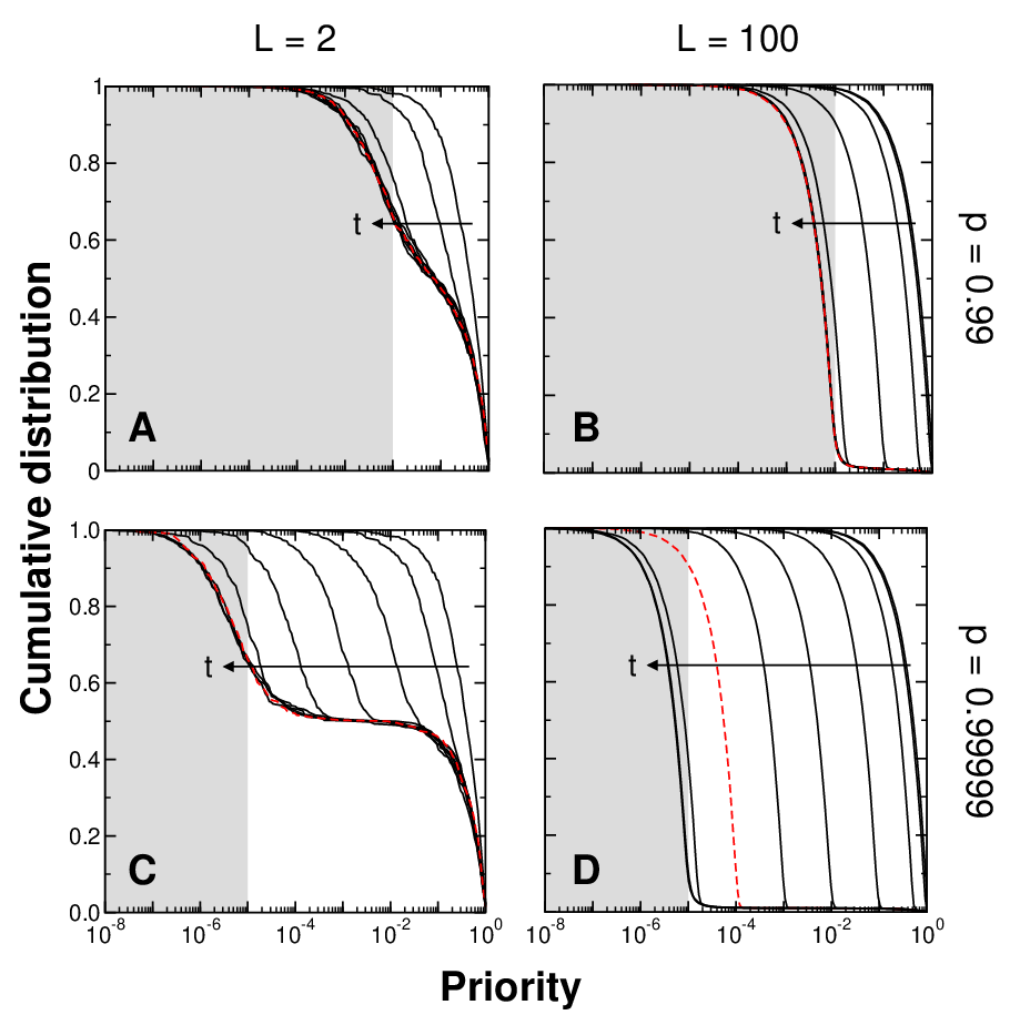
The priority queuing model also suffers from several unrealistic predictions. First, the time for the model to reach steady-state increases as Vázquez 2005. This means that for the case considered in Ref. Barabási 2005 (, ), the time to reach steady-state is on the order of tasks. If a user operating according to those parameter values sends 100 e-mails a day (a very large number of e-mails), it would take him 100,000 days 300 years to reach steady-state. It is also worthwhile to note that the results for the model in Ref. Barabási 2005 were not even obtained for steady-state, implying that the data is actually a mixture of different stages of the relaxation process of the model.
Second, after reaching steady-state, the dynamics of the model become quite anomalous. The priorities of the tasks in the user’s queue converge to a uniform distribution (Fig. 9), while new tasks arrive with a priority drawn from . Thus, in the limit , an e-mail user has a queue consisting of extremely low priority tasks and consequently performs new tasks with probability immediately upon arrival. This results in a peak at that accounts for nearly all of the probability mass (Fig. 10). Clearly this situation is not representative of e-mail activity, let alone human behavior as Ref. Barabási 2005 claims.

More fundamentally, the priority queuing model predicts a distribution of waiting times that decays as a power-law with an exponent Vázquez 2005; Vázquez et al. 2005 whereas the actual data clearly rejects that description; cf. Section IV. In fact, a superposition of two log-normals, one corresponding to waiting times of less than a day and another corresponding to a waiting time of several days provides an excellent description of the empirical data. More importantly, that description agrees with the common experience of e-mails users: one replies to e-mails within the day, if not, within the next few days, and if not then, never.
VI Conclusions
Here, we have quantitatively analyzed human e-mail communication patterns. In particular, we have found that the interevent times are well-described by a log-normal distribution while the waiting times are well-described by the superposition of two log-normal distributions. We have simultaneously rejected the hypothesis that either quantity is adequately described by a truncated power-law with exponent .
We have also critically examined the priority queuing model proposed by Barabási to match the empirically observed waiting time distributions. After detailed analysis, we conclude that neither the assumptions nor the predictions of the model are plausible. We note that the model does not match the empirically observed waiting time distribution, and we therefore contend that the theoretical description of human dynamics is an open problem.
Barabási and coworkers have also examined the dynamics of letter writing ao Gama Oliveira and Barabási 2005, web browsing, library loans, and stock broker transactions Vázquez et al. 2005. They argue that these processes also follow power-law distributions and are consequences of similar priority queuing processes. Our analysis demonstrates that care must be taken when describing data with fat-tails, particularly when the apparent scaling exponent is close to one and the probability distribution is concave.
Appendix A Maximum likelihood estimation
In maximum likelihood estimation, the likelihood function for distribution model given the data is
| (5) |
where is the number of data points in the sample, the are the empirical data points and is the probability density function for the candidate model evaluated at each empirical data point. We then maximize the likelihood to find the parametrization of the model distribution that best approximates the data. For the double log-normal model, double log-normal. To find the best estimate of the five parameters , we obtain preliminary estimates for and from the mean and standard deviation of and subsequently maximize likelihood to find the appropriate double log-normal parameters. In practice, however, one typically performs a minimization of Mood et al. 1974; Press et al. 2002.
References
- Stanley et al. (1996) M. H. R. Stanley, L. A. N. Amaral, S. V. Buldyrev, S. Havlin, H. Leschhorn, P. Maass, M. A. Salinger, and H. E. Stanley, Nature 379, 804 (1996).
- Amaral et al. (1997) L. A. N. Amaral, S. Buldyrev, S. Havlin, H. Leschorn, P. Maass, M. Salinger, and H. E. Stanley, J. Phys. I France 7, 635 (1997).
- Amaral et al. (1998) L. A. N. Amaral, S. V. Buldyrev, S. Havlin, M. A. Salinger, and H. E. Stanley, Phys. Rev. Lett. 80, 1385 (1998).
- Plerou et al. (1999) V. Plerou, L. A. N. Amaral, P. Gopikrishnan, M. Meyer, and H. E. Stanley, Nature 400, 433 (1999).
- Amaral et al. (2001) L. A. N. Amaral, P. Gopikrishnan, V. Plerou, K. Matia, and H. E. Stanley, Scientometrics 51, 9 (2001).
- Guimerà et al. (2002) R. Guimerà, A. Arenas, A. Díaz-Guilera, and F. Giralt, Phys. Rev. E 66, 026704 (2002).
- Smith (1786) A. Smith, An inquiry into the nature and causes of the wealth of nations (Methuen & Co., London, 1786).
- Pareto (1906) V. Pareto, Manuale di economia politica (Milano, Societa Editrice, 1906).
- Zipf (1949) G. K. Zipf, Human behavior and the principle of least effort: an introduction to human ecology (Addison-Wesley Press, Cambridge, MA, 1949).
- Ebel et al. (2002) H. Ebel, L.-I. Mielsch, and S. Bornholdt, Phys. Rev. E 66, 035103 (2002).
- Guimerà et al. (2003) R. Guimerà, L. Danon, A. Díaz-Guilera, F. Giralt, and A. Arenas, Phys. Rev. E 68, art. no. 065103 (2003).
- Eckmann et al. (2004) J.-P. Eckmann, E. Moses, and D. Sergi, Proc. Natl. Acad. Sci. USA 101, 14333 (2004).
- Barabási (2005) A.-L. Barabási, Nature 435, 207 (2005).
- Kossinets and Watts (2006) G. Kossinets and D. Watts, Science 311, 88 (2006).
- Berson (1992) A. Berson, Client/server architecture (McGraw-Hill, New York, NY, 1992).
- SkillCrest (2004) SkillCrest, VistaMetrix (2004), http://www.skillcrest.com/.
- Mood et al. (1974) A. M. Mood, F. A. Graybill, and D. C. Boes, Introduction to the Theory of Statistics (McGraw-Hill Companies, 1974).
- Bernardo and Smith (2000) J. M. Bernardo and A. F. M. Smith, Bayesian Theory (John Wiley & Sons, 2000).
- Vázquez et al. (2005) A. Vázquez, J. G. Oliveira, Z. Dezsõ, K.-I. Goh, I. Kondor, and A.-L. Barabási, arXiv:physics/050117 (2005).
- (20) A.-L. Barabási, K.-I. Goh, and A. Vazquez, Reply to Comment on ”The origin of bursts and heavy tails in human dynamics”.
- Vázquez (2005) A. Vázquez, Phys. Rev. Lett. 95, 248701 (2005).
- Miller (1956) G. A. Miller, Psych. Rev. 63, 81 (1956).
- ao Gama Oliveira and Barabási (2005) J. ao Gama Oliveira and A.-L. Barabási, Nature 437, 1251 (2005).
- Press et al. (2002) W. H. Press, S. A. Teukolsky, W. T. Vetterling, and B. P. Flannery, Numerical Recipes in C: The Art of Scientific Computing (Cambridge University Press, New York, 2002), 2nd ed.