Abstract
We present theoretical and numerical evidence to show that self-defocusing nonlinear optical propagation can be used to compute Euler fluid dynamics and possibly Navier-Stokes fluid dynamics. In particular, the formation of twin vortices and the Kármán vortex street behind an obstacle, two well-known viscous fluid phenomena, is numerically demonstrated using the nonlinear Schrödinger equation.
Metaphoric optical computing of fluid dynamics
Mankei Tsang and Demetri Psaltis
Department of Electrical Engineering, California Institute of Technology, Pasadena, California 91125
OCIS codes: (200.0200) Optical computing; (190.5530) Pulse propagation and solitons
1 Introduction
A Philosophy of metaphoric computing
Nonlinear dynamical systems, such as weather, plasma, and the economy, are ubiquitous in nature and everyday’s life, yet such systems are typified by their highly complex and chaotic behaviors, making them notoriously difficult to study theoretically, experimentally, and numerically. Analytic solutions of nonlinear systems are rare, experiments are often too inflexible or impractical, and numerical simulations must take into account a large number of data points in multiple dimensions in order to accurately model a problem of interest, such that even the fastest supercomputers today would take days or weeks to simulate relatively simple nonlinear dynamics that a physical system exhibits in seconds.
On the opposite side of the same coin, we can regard the physical system as a computational device that computes its own dynamics at a speed unimaginable by supercomputers. The key to harnessing this tremendous computing power of a physical system is therefore to make it compute other interesting problems of the same order of complexity. Of course, a conventional digital computer is itself a physical system, but it makes use of complex semiconductor physics to compute elementary logic operations, and in doing so, discards a large amount of information that is considered extraneous. In this perspective, a digital computer is an extremely inefficient computing device, as it only utilizes an exceedingly small amount of the full computing capability potentially offered by its physics. The advantage in this case is the flexibility in cascading different logic operations for general-purpose computing, but as evidenced by the difficulties in the numerical simulations of nonlinear dynamical systems, this inefficient computing method is often inadequate.
In order to make full use of the computing capability offered by a physical system, we hereby propose the concept of metaphoric computing, which makes use of a more experimentally accessible nonlinear dynamical system to simulate another nonlinear dynamical system. An example of this computing method is a wind tunnel, in which a small-scale fluid experiment is performed to simulate large-scale fluid dynamics, by virtue of the scaling laws inherent in fluid dynamics. Metaphoric computing, however, is not restricted to the use of similar physical systems to simulate each other. In this paper, we show in particular that nonlinear optics can compute fluid dynamics as well. An optical beam inherently holds three-dimensional spatiotemporal information, and nonlinear optical propagation computes the evolution of this large amount of information simultaneously at the speed of light, promising substantial parallelism and speed for computing. Although the use of nonlinear optics for digital computing has not been as successful as the use of solid-state electronics, forcing optical beams to compute binary logic wastes most of the spatiotemporal information that can be manipulated in optical beams. Instead of fitting a square peg in a round hole, using optics to simulate other nonlinear dynamical systems provides a natural way of making full use of the computing capacity offered by a nonlinear optical system.
Fluid dynamics, the foundation of a wide variety of important research fields including meteorology, aeronautics, plasma physics, superfluids, and Bose-Einstein condensates, is an ideal problem to solve by metaphoric computing. Intractable theoretical analysis and inflexible experiments compel the use of numerical simulations, the difficulty of which nonetheless gives rise to a whole new field, computational fluid dynamics, in itself. The main difficulty is due to the inherent complexity of a fluid dynamics problem, which is nonlinear and continuously generates finer structures as the fluid dynamics evolves. For problems that are of practical interest, such fine structures are often orders-of-magnitude smaller than the size of the objects under consideration, thus requiring a large number of data points in each of the three spatial dimensions to be manipulated at each time step, which must also be correspondingly small to avoid numerical instabilities. An alternative method of simulating complex fluid dynamics that combines the speed of a fluid experiment and the flexibility of a numerical analysis is hence of great practical importance. In this paper, we show that, via a suitable transformation, nonlinear optical propagation can be utilized to simulate Euler fluid dynamics, which is known to be computationally expensive and unstable to solve numerically . We also provide strong evidence that nonlinear optics can simulate high-Reynolds-number Navier-Stokes fluid dynamics as well, which include a large class of important and computationally difficult problems, such as turbulence. With the speed, parallelism, and configurability of optics, an “optical wind tunnel” may one day become a viable alternative to experiments and numerical analysis in the study of fluid dynamics.
B Correspondence between nonlinear optics and fluid dynamics
The analogy between nonlinear optics and fluid dynamics has been noted by many authors [1, 2, 3, 4, 5, 6, 7, 8, 9, 10, 11, 12, 13, 14, 15, 16, 17, 18]. Wagner et al. first suggested that the nonlinear propagation equation of an optical beam can be recast into equations that resemble the continuity equation and the Bernoulli equation in irrotational fluid dynamics [1]. Coullet et al. first coined the term “optical vortices,” which shows the analogy between phase singularities in optics and fluid vortices [2]. Brambilla et al. noted that laser equations can be transformed to a hydrodynamic form [3]. Arecchi et al. first experimentally demonstrated the dynamics of optical vortices in nonlinear optics [4]. Akhmanov et al. called the rich nonlinear dynamics observed in a nonlinear resonator “optical turbulence.” [5] Swartzlander and Law observed optical vortex solitons created via the instability of dark soliton stripes analogous to the Kelvin-Helmholtz instability in fluid dynamics [6]. Staliunas showed that a laser can be described by the Ginzburg-Landau equation, which can be transformed into equations resembling the Navier-Stokes equations that describe viscous fluid dynamics [7]. Vaupel et al. observed vortex pair nucleation by the interference of two modes in a laser and claimed that it was an analog of a vortex street behind an obstacle in a fluid flow [8]. Molina-Terriza et al. also observed optical vortex streets in walking second-harmonic generation [9]. Roux [10] and Rozas et al. [11] studied the interactions between optical vortices and found that their interactions resemble those of fluid vortices. Rozas et al. then experimentally demonstrated the fluidlike motion of a pair of optical vortices [12]. Michinel et al. [13] and Paz-Alonso et al. [14] found that optical propagation in a cubic-quintic nonlinear medium resembles a liquid drop, and optical vortices in such a medium also have fluidlike motions [15]. On the other hand, nonlinear optics has been compared with superfluids and Bose-Einistein condensates, as they can all be described, to varying degrees, by the nonlinear Schrödinger equation [19, 20], commonly known as the Gross-Pitaevskii equation in the field of superfluids [21]. Pomeau and Rica suggested that the phenomenon of transition to dissipation in a superflow [22] can be observed in nonlinear diffraction [16]. Bolda et al. numerically demonstrated the same phenomenon in a nonlinear Fabry-Pérot cavity [17]. Chiao also found that photons in such a cavity should obey the Bogoliubov dispersion relation for a superfluid [18].
The abundant amount of prior work credited above provides ample evidence that nonlinear optics resembles fluid dynamics to a certain degree. In order to use nonlinear optics as a useful and practical computational tool for fluid dynamics, however, simply drawing analogies between the two kinds of dynamics is not enough. One must be able to show an exact correspondence, or at the very least, an approaching convergence between a problem in nonlinear optics and a problem in fluid dynamics, in order to produce any useful prediction of fluid dynamics via nonlinear optics. Moreover, as computers nowadays have enough capabilities to simulate two-dimensional fluids, the mere correspondence between optics and two-dimensional fluid dynamics considered in most of the prior work would not motivate the use of metaphoric optical computing in preference to conventional digital computing. A three-dimensional fluid modeling, on the other hand, requires a processing capability orders-of-magnitude higher than that available in today’s supercomputers, so metaphoric optical computing would need to compute such problems much more efficiently to compete with electronic computers and the Moore’s law.
In the following sections, we shall attempt to establish the correspondence between nonlinear optics and three-dimensional fluid dynamics. We shall show that, taking group-velocity dispersion into account, nonlinear optical dynamics approaches three-dimensional inviscid Euler fluid dynamics in the highly nonlinear self-defocusing regime, where the optical intensity represents the fluid density, the optical phase gradient represents the fluid velocity, the nonlinear refractive index perturbation represents pressure, the propagation distance represents time, and the temporal dimension of the optical pulse represents the third dimension of the fluid. As Euler fluid equations often exhibit high numerical instabilities, this correspondence in itself should be useful in modeling high-Reynolds-number fluid dynamics away from objects and boundaries. In the convergence of nonlinear Schrödinger equation towards the Euler equations, a “quantum pressure” term arising from the nonlinear Schrödinger equation plays the role of a small parameter. As this quantum pressure term plays analogous roles to viscosity in the Navier-Stokes equations, we argue that nonlinear optics should be able to approximate viscous Navier-Stokes fluid dynamics as well, in the regime where quantum pressure and viscosity both play the role of small parameters in the respective equations. That said, we do not pretend that we have established the equivalence between nonlinear optics and Navier-Stokes dynamics, as the similarity between quantum pressure and viscosity is still an open problem.
On the practical side, in cases where ideal nonlinear optics setup is not available, we suggest a split-step method that pieces together different optical devices to approximate an ideal nonlinear optics experiment. This method is very similar to the method proposed to simulate quantum systems using a quantum computer [23].
It must be stressed that although we focus on simulations of classical physical systems, future quantum computers that simulate quantum systems [23] would run into the same problem of manipulating a large amount of multi-dimensional information. In the case of quantum systems, multi-dimensional quantum information, such as a multi-particle multi-spatiotemporal-dimensional wavefunction, needs to be processed in parallel. Quantum computers can naturally parallelize the multi-particle aspect, but there is no obvious way of parallelizing the manipulation of multi-spatiotemporal-dimensional information via simple binary quantum logic. Perhaps a quantum metaphoric computing would then be necessary, where a more accessible multi-dimensional quantum system is used to simulate another quantum system.
2 Correspondence between nonlinear optics and Euler fluid dynamics
A Madelung transformation
We now proceed to show mathematically how the self-defocusing nonlinear optical propagation equation, including the effect of group-velocity dispersion, can be transformed to three-dimensional hydrodynamic equations. First, we show how the optics equations, in the absence of optical vortices, correspond to inviscid and irrotational fluid equations. This form of transformation is widely attributed to Madelung [24]. We model the paraxial nonlinear propagation of an optical beam, described by the envelope function , via the nonlinear Schrödinger equation [19, 20],
| (1) |
where is the propagation distance, is the carrier wave number, is the group-velocity dispersion coefficient, is the time coordinate in the moving frame of the pulse, and is the nonlinear Kerr coefficient. To use the time coordinate as the third spatial dimension of a fluid, anomalous group-velocity dispersion, or , is required. Dispersion can then be regarded in equal footing as diffraction if a normalized time coordinate is defined as
| (2) |
such that
| (3) |
The Madelung transformation is defined as follows,
| (4) | ||||
| (5) | ||||
| (6) |
such that the evolution equations for the intensity, , and the phase gradient, , are given by
| (7) | ||||
| (8) |
One can already see that Eq. (7) has the exact same form as the fluid continuity equation, while Eq. (8) resembles the Bernoulli equation [1], if one regards the intensity as the fluid density and the phase gradient as the fluid velocity. The nonlinear refractive index term, , would resemble the fluid pressure if , so self-defocusing is required. The last term in Eq. (8) is a peculiar term that arises from optical diffraction and dispersion, does not exist in classical fluid dynamics, and is commonly called the “quantum pressure.”
In order to compare these equations with fluid equations more easily, we use the following normalized variables,
| (9) | |||
| (10) | |||
| (11) |
where is the characteristic size, is the characteristic phase gradient, is some characteristic optical intensity of the propagation, and is the so-called “healing” length, which is the length scale at which the quantum pressure term has the same order of magnitude as the nonlinear term on the right hand side of Eq. (8), is the Mach number, which measures the relative strength of fluid pressure compared with convection, and is another number that measures the relative strength of fluid convection compared with quantum pressure. The normalized equations become
| (12) | ||||
| (13) |
Equation (12) is exactly the same as the fluid continuity equation, and in the limit of , which is the highly self-defocusing regime, Eq. (13) is the same as the hydrodynamic equation of motion that describes inviscid and irrotational fluids. Equations (12) and (13) also admit sound wave solutions, which describe travelling perturbations to the density and the velocity. As long as the sound waves are weak, the dependence of pressure on the density is not crucial, and the use of self-defocusing Kerr nonlinearity is adequate. This restricts the correspondence to slightly compressible barotropic fluids.
In order to model slightly compressible fluids, the optical beam needs to have a relatively constant intensity background. This can be achieved approximately near the center of a very large beam, in a large multimode waveguide as a container in two spatial dimensions, or in a cubic-quintic nonlinear medium to provide a “surface tension” to the beam [25, 13, 14, 15].
B Vorticity
In general, the fluid velocity vector should contain an irrotational component and a rotational component,
| (14) |
where is called the velocity potential, and the curl of is defined as the fluid vorticity,
| (15) |
The dynamics of vorticity is arguably the cornerstone of hydrodynamics [21]. The inviscid fluid dynamics that includes the rotational effect is governed by the Euler equation,
| (16) |
where is the pressure. For incompressible fluids, , and as long as increases with , the specific dependence of on the fluid properties is not important. Equation (16) contains the convective term , which can be written as
| (17) | ||||
| (18) |
One can then see that the optical Bernoulli equation, Eq. (13), misses the rotational component of the convective term. In other words, the Madelung transformation is only able to describe the irrotational part of the fluid motion, but not the more important rotational part.
The inability of the Madelung transformation to describe vorticity is due to the failure of the transformation near optical vortices, where Eq. (13) is ill-defined. To understand this problem, consider a rectilinear optical vortex in polar coordinates and neglect the third fluid dimension for now,
| (19) | |||
| (20) |
where is an integer and is called the topological charge of an optical vortex. The phase gradient is then given by
| (21) |
The fluid vorticity is proportional to the curl of ,
| (22) |
which resembles the vorticity of an ideal point fluid vortex [26]. The motion of these vortices, however, cannot be described by the Madelung transformed equations due to two problems: diverges when , so the fluid velocity at the center of a vortex is infinite, and must approach in the limit of to maintain the continuity of , so the quantum pressure term, with in the denominator, is also infinite near the vortex center.
To overcome these difficulties, it is necessary to consider the motion of the optical vortices separate from the irrotational optical flow.
C Optical vortex solitons and point vortices
In a relatively constant intensity background, optical vortices exist as optical vortex solitons [27, 6, 25]. The optical envelope function of a vortex soliton is given by Eq. (19), where for , and approaches a constant for , where is the healing length and also the size of the dark spot of a vortex soliton. In three dimensions, a vortex soliton exists as a vortex filament. We shall hereafter consider single-charged vortex solitons with only, as they have the lowest energy and are the most prevalent ones arising from an experimental situation. It is also more accurate to approximate continuous vorticity with only discrete vortices with the smallest topological charge.
Eq. (22) suggests that an optical vortex soliton resembles an ideal point vortex in incompressible fluids. Indeed, the motion of optical vortices in the highly self-defocusing limit can be rigorously proven to behave in the same way as point fluid vortices [10, 11, 28, 29, 30, 31]. If one defines the position of each vortex filament as , then the fluid velocity at each point due to the presence of the vortex filaments in the limit of high self-defocusing is given by
| (23) |
where is the normalized three-dimensional position vector, is the topological charge of vortex , and describes the irrotational flow according to Eq. (13). In particular, the motion of each filament is given by,
| (24) |
in the leading order. These equations of vortex motion are valid as long as the separations of the vortices are much larger than . For example, Fig. 1 plots the intensity, phase, and phase gradient of two rectilinear optical vortex solitons with the same charge, which should rotate around each other, and those of two vortices with opposite charges, which should drift in the same direction perpendicular to their separation.

With the vortex filaments, one can define the equivalent vorticity in an optical beam,
| (25) |
which can be used to approximate the continuous vorticity of a fluid, if the number of vortex filaments is large enough. In this case, to include the vorticity effect in the nonlinear optical dynamics, one can phenomenologically patch up the irrotational equation of motion, Eq. (13),
| (26) |
This modification of the equation of motion can be attributed to the phenomenon of phase slippage [21, 32], well known in the field of superfluids. The use of discrete point vortex interactions to calculate Euler fluid dynamics is also a well-known numerical method in computational fluid dynamics [33]. Hence, to simulate Euler fluid dynamics, one can approximate both the rotational and irrotational components of the initial fluid velocity profile by the optical phase and the phase singularities in an optical beam, and the nonlinear self-defocusing propagation of the beam would converge to incompressible Euler fluid dynamics in the strongly self-defocusing regime. One can also borrow from the well-established numerical techniques [33] to determine how the distribution of optical vortices sufficiently approximates the continuous vorticity in fluids.
D The fluid flux representation
So far, we have shown that optical vortex solitons behave like point vortices in fluids when they are far away from each other, and this behavior can be used to approximate Euler fluid dynamics. However, there is no guarantee that the vortices would remain well separated in the course of the vortex dynamics. If optical vortices behaved exactly like point vortices, then their velocities would diverge when they are close to each other. This velocity divergence is well known to cause significant numerical instability in the use of point vortices for computational fluid dynamics [33]. Another problem is that in three dimensions, the self-induced velocity of a curved point vortex filament diverges logarithmically in the limit of [33]. Since the optical intensity decreases to zero near the center of an optical vortex, the quantum pressure term, which determines the size of the vortex dark spot, can no longer be ignored, and the optical vortex interactions should differ markedly from point vortex interactions when their separation is on the order of .
To investigate the optical vortex dynamics when they are close to each other, the fluid velocity is no longer an appropriate quantity to study, because it diverges near a vortex center. The density, on the other hand, approaches zero towards the center. This motivates us to define an alternative finite quantity by multiplying the velocity and the density,
| (27) |
which is the fluid flux, or the momentum density. Simple calculations show that the flux is indeed finite everywhere in an optical beam, including the center of an optical vortex. In terms of the flux, the tensor dynamical equations now read [34]
| (28) | ||||
| (29) |
where is the th component of , is the th spatial derivative, and repeated indices are implicitly summed in the manner of Einstein’s summation. These equations have the same form as the normalized Euler equations in the tensor form,
| (30) | ||||
| (31) |
except the quantum pressure term in Eq. (29). Hence, in the flux representation, we have successfully avoided the problem of divergent quantities. Furthermore, Eq. (29), in contrast to Eq. (13), includes the correct convective term.
The use of momentum density in the description of nonlinear optical dynamics is more natural and appropriate than the use of velocity in the Madelung transformation, as the dynamics ultimately evolves according to the basic law of momentum conservation. As we shall show next, when comparing the optical flux to the fluid flux, the dynamics of optical vortex solitons are much more similar to that of less singular fluid vortices than point vortices, and the correspondence between nonlinear optics and Euler fluid dynamics is still justified when is finite.
E Optical vortex solitons and vortex blobs
In light of the fluid flux representation, one should therefore compare the flux of an optical vortex soliton to the flux of a fluid vortex. In an incompressible fluid, the density is constant, so the flux is proportional to the velocity, and the flux at the center of a point vortex has the same singular behavior as the velocity. Near a vortex soliton, however, the flux is finite. Consider the example of a single-charged vortex soliton. The flux near the center is given by
| (32) |
which vanishes as , as opposed to the divergence of at the center of a point vortex.
Instead of comparing a vortex soliton to a point vortex, one should hence compare the soliton to a vortex blob [33], which has finite vorticity over a finite area. The vorticity of a vortex blob filament is mathematically described by
| (33) |
where is a vorticity distribution function for the filament. The velocity near the center of a rectilinear vortex blob and far away from the center is
| (34) | |||
| (35) |
so in an incompressible fluid, the fluid flux of an optical vortex soliton with size is the same as that of a vortex blob with size . See Fig. 2 for a graphical illustration.

The dynamics of a vortex blob and that of a vortex soliton are also extremely similar. For example, the rotation frequency of two like-charged vortex blobs approaches a constant when their separation goes to zero. Numerical simulations of the nonlinear Schrödinger equation also show that the rotation frequency of two like-charged vortex solitons approaches a constant and does not diverge like two point vortices [35]. On the other hand, the self-induced velocity of a curved vortex blob filament is given by [33]
| (36) |
where is the unit binomial vector of the filament and is the radius of curvative. The self-induced velocity of an optical vortex soliton filament is proven to be exactly the same [29]. Hence, optical vortex solitons act as vortex blobs, and a large number of solitons can simulate Euler fluid dynamics, much like the popular discrete vortex blob method in computational fluid dynamics [33].
F Numerical evidence of correspondence between nonlinear optics and Euler fluid dynamics
The most telling evidence of the correspondence between nonlinear optics and Euler fluid dynamics is perhaps the numerical fluid dynamics simulations using the nonlinear Schrödinger equation by Nore et al. [36, 37]. Using the nonlinear Schrödinger equation, Nore et al. numerical demonstrated the Euler fluid dyanmics of a jet made of an array of counter-rotating vortices, which exhibit sinuous and varicose instabilities [36]. In another study, Nore et al. also demonstrated three-dimensional shear flows and showed that numerically solving nonlinear Schrödinger equation is a viable alternative to Euler and Navier-Stokes equations for the numerical study of shear flows [37]. As nonlinear optical propagation is governed by nonlinear Schrödinger equation, The numerical experiments by Nore et al. show that nonlinear optics should also be able to compute Euler fluid dynamics.
3 Similarities between nonlinear Schrödinger dynamics and Navier-Stokes fluid dynamics
In the previous sections, we have shown the correspondence between self-defocusing optical propagation and inviscid Euler fluid dynamics via a variety of methods, including the Madelung transformation, the incorporation of vorticity effect due to the “phase slip” phenomenon, the fluid flux representation, and the comparison between optical vortex solitons and vortex blobs. Even though viscosity plays the role of a small parameter in most interesting fluid dynamics problems, its effects are of paramount importance near a “no-slip” boundary and in the dissipation of eddies, in which cases the viscous Navier-Stokes equations should be used. In this section we shall present evidence that the nonlinear Schrödinger equation exhibits many of the same behaviors of viscous Navier-Stokes fluid dynamics, and in each case, quantum pressure plays an analogous role to viscosity.
The normalized Navier-Stokes equations in the flux representation are given by
| (37) | ||||
| (38) |
where the last term in Eq. (38) is the viscosity term and is called the Reynolds number, which describes the relative strength of convection compared to viscosity,
| (39) |
where is the characteristic velocity of the fluid system, is the characteristic length, and is the kinematic viscosity of the fluid. Comparing the viscosity term in Eq. (38) with the quantum pressure term in Eq. (29) via a dimensional analysis would suggest that an analogous optical Reynolds number would be defined as
| (40) |
where, to recall, is the characteristic optical phase gradient, and is the characteristic size of the optical experiment setup. The optical Reynolds number thus roughly measures the number of optical vortices. In other words, if the optical Reynolds number indeed corresponds to its fluid counterpart, then the quantization of the optical vortices would play an analogous role to fluid viscosity. This view seems to be echoed by other researchers in the field of superfluids [38, 39, 40, 41], although we must stress that it is still an open problem as to what extent the quantization effect resembles the viscous effect [41].
A Zero-flux boundary conditions, boundary layers, and boundary layer separation
In classical fluid dynamics the “no-slip” boundary condition is most commonly used, and restricts the total velocity and hence the total flux to be zero at the boundary. For fluid flow above a surface, the velocity shear introduced must be balanced by a viscous stress, resulting in a boundary layer that connects the zero velocity at the boundary to the flow velocity above the boundary in an asymptotic expansion [42]. For the nonlinear Schrödinger equation, the boundary condition of an impenetrable object can be specified by a very low refractive index region, which restricts the optical intensity to be zero at the surface [43] due to total internal reflection. Even though the tangential velocity can have a non-zero value at the surface, both the normal and tangential components of the flux must be zero there. This can hence be viewed as a zero-flux “no-slip” boundary condition. An optical boundary layer analogous to the viscous boundary layer in classical fluid dynamics is also formed [43]. See Fig. 3 for a graphical illustration of the similarities between a viscous boundary layer and an optical boundary layer.

For a viscous fluid flow past an obstacle, as the Reynolds number increases, the boundary layer begins to separate and vorticity is convected behind the obstacle. An analogy in the dynamics of the nonlinear Schrödinger equation, in the form of vortex nucleation on the boundary, is also predicted [22], and in the case of large objects, the instability of the optical boundary layer also depends on the optical Reynolds number defined in Eq. (40) [40], much like the viscous boundary layer separation.
B Dissipation of eddies
Another important effect of viscosity is the dissipation of small-scale structures in turbulence. An analogous effect in nonlinear Schrödinger equation is the emission of sound waves two vortices are close to each other [35] and the generation of Kelvin waves in the process of vortex line reconnections [44]. The radiation of acoustic energy in both cases must cause a damping of the high-spatial-frequency convection within the optical beam, and the effective Reynolds number is again estimated to be equal to the optical Reynolds number [38, 39, 41].
C Kármán vortex street
The Kármán vortex street is a famous viscous fluid phenomenon, in which alternate fluid vortices are emitted from the back of an obstacle to the flow of a viscous fluid, when the Reynolds number increases beyond a certain threshold [26, 45]. Using the numerical vortex blob method, Chorin first simulated such a phenomenon for a cylinder obstacle and obtained good agreement with experimental data [46]. Since an optical beam diffracting past a low refractive index region would also emit optical vortices and the vortices interact like vortex blobs in a self-defocusing medium, we performed a numerical experiment of the nonlinear Schrödinger equation to investigate if we would observe a similar phenomenon for nonlinear optics.

The numerical setup is sketched in Fig. 4. A big optical beam is assumed to propagate at an angle to an ellipsoid cylinder, with a refractive index much lower than the surroundings to act as an impenetrable object, in a self-defocusing medium. The length of the long axis of the ellipsoid cross section is assumed to be , and the short axis is assumed to be one-fifth of throughout the simulations. The two-dimensional nonlinear Schrödinger equation is solved using the Fourier split-step method [20], which implies a periodic boundary condition for the optical beam. This should not affect the qualitative behavior of the dynamics, if the optical beam is much bigger than the object. In all of the simulations, the Mach number is fixed at 0.4, while the optical Reynolds number is varied. Figure 5 plots the intensity of the optical beam at a normalized propagation distance for an optical Reynolds number . Optical vortex solitons are created on the top and bottom side of the low-refractive-index region, and they interact in such a way that resembles the phenomenon of twin vortices behind an obstacle in a low-Reynolds-number viscous fluid flow.

Figure 6 plots the flux and Fig. 7 plots the momentum vorticity . Both plots confirm the similarity between the numerically observed dynamics and the phenomenon of twin vortices in a viscous fluid flow.


Figures 8, 9, and 10 plot the intensity, flux, and momentum vorticity of the optical beam respectively, at a longer propagation distance for the same parameters. The qualitative dynamical behavior of vortices staying behind the object is essentially unchanged.


We now raise the Reynolds number to and perform the numerical experiment again. As seen from Figs. 11, 12, and 13, the optical vortex solitons become smaller and more abundant, but at the phenomenon of twin vortices behind an obstacle is again observed.


At , however, significant instability in the twin vortices develops, such that the spatial symmetry between the upper plane and the lower plane is broken, and alternative bunches of optical vortices begin to be emitted from the back of the object. Figures 14, 15, and 16 plot the intensity, flux and vorticity at respectively, which demonstrate a behavior strongly resembling the famous Kármán vortex street phenomenon.


Due to computing power constraints, we are only able to simulate low-Reynolds-number flows, which we do not expect to quantitatively reproduce viscous fluid dynamics. We have to use an ellipsoid cylinder in the numerical experiments, instead of the more conventional circular cylinder, to artificially generate more optical vortices, and the Mach number is a little too high for compressional waves not to play a significant role in the dynamics. With all that said, using the nonlinear Schrödinger equation, we are still able to qualitatively demonstrate, for the first time to our knowledge, two well-known viscous fluid phenomena, namely, the formation of twin vortices behind an obstacle, and the symmetry-breaking instability of the twin vortices that leads to the Kármán vortex street when the Reynolds number is increased. Compared with previous claims of observing the Kármán vortex street in nonlinear optics numerically [7] or experimentally [8, 9], our numerical results demonstrate an unprecedented level of correspondence between nonlinear optical dynamics and the Kármán vortex street phenomenon, thanks to the presence of a much larger number of optical vortices in our simulations.
D Kolmogorov turbulence
The striking similarities between nonlinear optics and viscous fluid dynamics are not limited to low-Reynolds-number two-dimensional problems. As the Reynolds number is further increased to the order of a million, the viscous fluid flow enters a turbulent regime. Since this regime is highly chaotic, only statistical signatures can be reproduced in a turbulent fluid flow. A well-known signature of turbulence is the Kolmogorov energy spectrum [47], derived under the assumption that a “steady state” is reached when the macroscopic-scale fluid flow continuously generate finer spatial structures via convection and viscosity dissipates the smallest structures. As viscosity plays a significant role in the Kolmogorov turbulence spectrum, it is surprising to see that numerical simulations of the three-dimensional nonlinear Schrödinger equation also reproduce the Kolmogorov spectrum at high Reynolds numbers, and the vorticity dynamics of the “superflow” described by the nonlinear Schrödinger equation resembles that of the viscous flow, in which vortex reconnection events play a major role [38, 39].
The dissipation of the smallest spatial structures in a superflow is speculated to be the Kelvin waves produced by the natural motion and reconnections of vortex filaments [41, 44], and the corresponding Reynolds number is again speculated to be [41]. Numerical and theoretical analyses of the so-called “quantum turbulence” exhibited by the nonlinear Schrödinger equation all reveal striking similarities between quantum and classical fluids, and it is argued that the study of quantum turbulence could lead to a better understanding of turbulence in normal fluids [48].
4 The split-step method
While a nonlinear optical system shows promise for computing Euler and Navier-Stokes fluid dynamics, it also poses serious technical challenges. Ideally one would like to have a configurable nonlinear material with low loss, anomalous group-velocity dispersion, high defocusing nonlinearity, and three-dimensional co-propagating boundaries. One may only be able to find separate materials or optical devices, each of which performs only some of the functions. Moreover, parasitic effects such as loss, two-photon absorption, and high-order dispersion can be detrimental to the accuracy. To combine different devices and periodically compensate for parasitic effects, we hereby propose the “split-step” method, the inspiration of which comes from the numerical Fourier “split-step” method [20]. Consider the general nonlinear Schrödinger equation,
| (41) |
where propagation effects and boundary conditions are expressed in terms of operators . The formal solution is
| (42) |
But if is much smaller than where is the magnitude of the operators, by virtue of the Baker-Hausdorff formula we have
| (43) |
Each of the propagation effects can hence be applied separately to an optical pulse, with a quadratic error term. A symmetrized version of the split-step method can further reduce the error order,
| (44) |
The split-step method is not unlike the proof of a quantum computer being able to simulate any quantum systems [23]. Whereas it is difficult to find a quantum device that performs the exact Hamiltonian of the quantum system of interest, it is possible to approximate the Hamiltonian in small time slices. Similarly, in a metaphoric optical computer, one can form a unit cell of a “meta-material” by combining a slice of defocusing material, a slice of material with anomalous group-velocity dispersion, a slice of ultrafast phase modulator to apply the three-dimensional boundary conditions, and a gain medium to compensate for loss. The optical beam can loop through the unit cell multiple times in a cavity, so that the outcome will approximate the true solution as if we had an ideal medium. See Fig. 17 for a graphical illustration of the method.
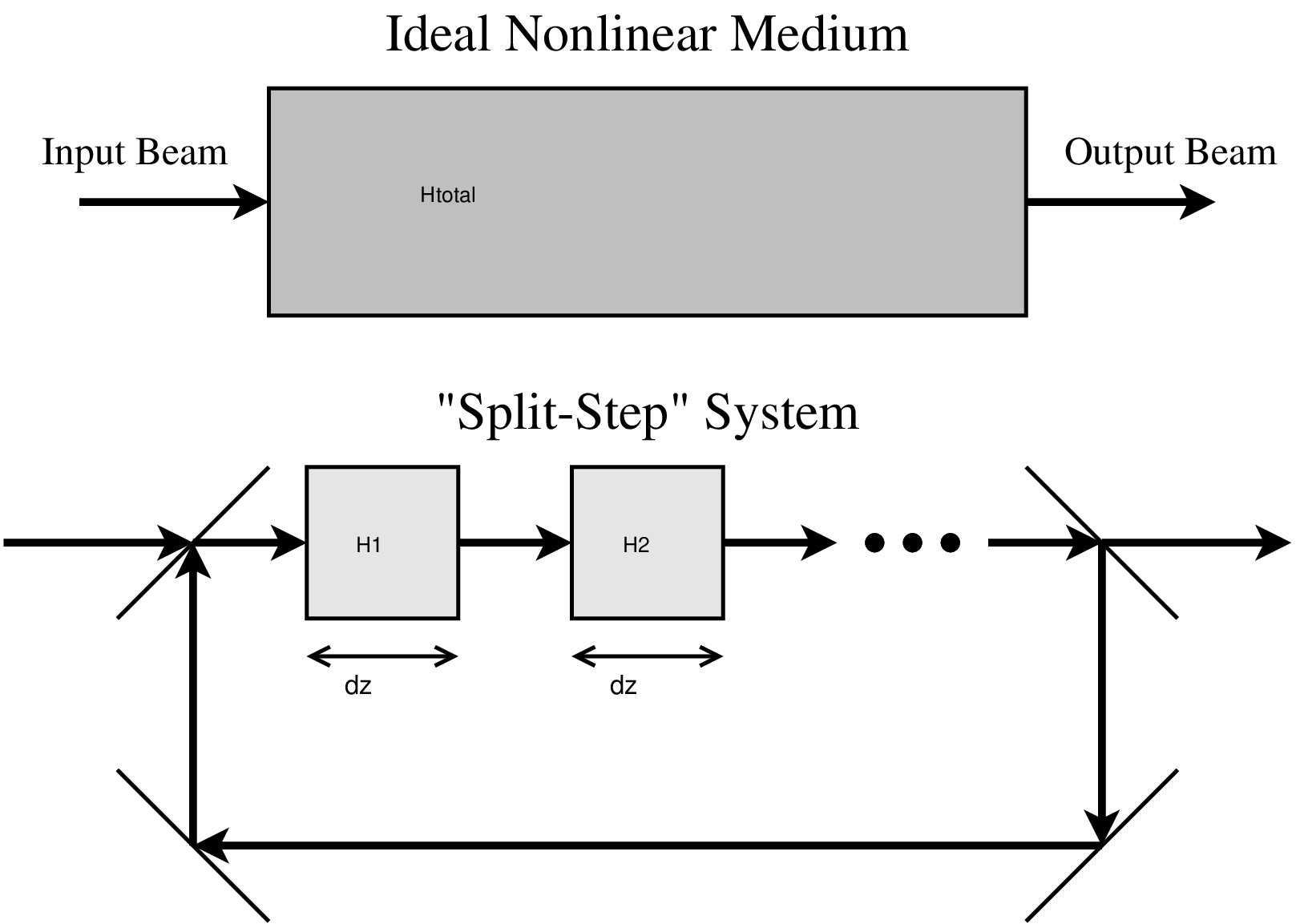
The split-step method has the additional advantages that each subsystem can be tunable and easily substituted with another material or device, and the pulse evolution can be monitored more easily. The magnitude of each effect can be tuned by simply changing the propagation length in each device, In exchange of configurability we have sacrificed some accuracy due to discretization errors and instability. The computation speed may also be reduced by a large but constant fraction, as the pulse may spend most of its time on simply propagating from one device to the next and not performing the core computation by nonlinear propagation. The split-step method, however, does not detract from the inherent parallelism in the computation, as the transverse dimensions are not discretized.
5 Conclusion
In conclusion, we have used a variety of theoretical and numerical methods to show that self-defocusing optical propagation has a converging correspondence with Euler fluid dynamics and a striking similarity with Navier-Stokes fluid dynamics. We have numerically shown that the interactions of a large number of optical vortex solitons are able to simulate two well-known viscous fluid phenomena. We have also proposed the split-step method, a way of practically implementing the metaphoric optical computer.
There are serious technical challenges if a metaphoric computer is to become useful for computing fluid dynamics, especially three-dimensional fluid dynamics problems, as techniques for the complete specification and characterization of the spatiotemporal optical field are still in their infancy. The speed, configurability, and parallelism of a metaphoric optical simulator nonetheless promise vast advantages over conventional numerical simulations.
Since photons are quantum objects, optical propagation would also inherently compute the quantum dynamics of bosons, and may therefore be used as a metaphoric simulator of quantum fluids, such as superfluids, superconductors, and Bose-Einstein condensates. In this way the advantages of a metaphoric computer and those of a quantum computer are combined, and only then the classical and quantum computing capabilities offered by photons would truly be exhausted. This extension of metaphoric optical computing will be a subject of future work.
Acknowledgments
We would like to acknowledge helpful and inspiring discussions with Ravi Athale, Michael C. Cross, and Martin Centurion. This work is supported by the Defense Advanced Research Projects Agency (DARPA).
References
- [1] W. G. Wagner, H. A. Haus, and J. H. Marburger, “Large-scale self-trapping of optical beams in the paraxial ray approximation,” Phys. Rev. 175, 256-266 (1968).
- [2] P. Coullet, L. Gil, and F. Rocca, “Optical vortices,” Opt. Commun. 73, 403-408 (1989).
- [3] M. Brambilla, L. A. Lugiato, V. Penna, F. Prati, C. Tamm, and C. O. Weiss, “Transverse laser patterns. II. Variational principle for pattern selection, spatial multistability, and laser hydrodynamics,” Phys. Rev. A 43, 5114-5120 (1991).
- [4] F. T. Arecchi, G. Giacomelli, P. L. Ramazza, and S. Residori, “Vortices and defect statistics in two-dimensional optical chaos,” Phys. Rev. Lett. 67, 3749-3751 (1991).
- [5] S. A. Akhmanov, M. A. Vorontsov, V. Yu. Ivanov, A. V. Larichev, and N. I. Zheleznykh, “Controlling transverse-wave interactions in nonlinear optics: generation and interaction of spatiotemporal structures,” J. Opt. Soc. Am. B 9, 78-90 (1992).
- [6] G. A. Swartzlander, Jr. and C. T. Law, “Optical vortex solitons observed in Kerr nonlinear media,” Phys. Rev. Lett. 69, 2503-2505 (1992).
- [7] K. Staliunas, “Laser Ginzburg-Landau equation and laser hydrodynamics,” Phys. Rev. A 48, 1573-1581 (1993).
- [8] M. Vaupel, K. Staliunas, and C. O. Weiss, “Hydrodynamic phenomena in laser physics: Modes with flow and vortices behind an obstacle in an optical channel,” Phys. Rev. A 54, 880-892 (1996).
- [9] G. Molina-Terriza, D. V. Petrov, J. Recolons, and L. Torner, “Observation of optical vortex streets in walking second-harmonic generation,” Opt. Lett. 27, 625-627 (2002).
- [10] F. S. Roux, “Dynamical behavior of optical vortices,” J. Opt. Soc. Am. B 12, 1215-1221 (1995).
- [11] D. Rozas, C. T. Law, and G. A. Swartzlander, Jr., “Propagation dynamics of optical vortices,” J. Opt. Soc. Am. B 14, 3054-3065 (1997).
- [12] D. Rozas, Z. S. Sacks, and G. A. Swartzlander, Jr., “Experimental observation of fluidlike motion of optical vortices,” Phys. Rev. Lett. 79, 3399-3402 (1997).
- [13] H. Michinel, J. Campos-Táboas, R. García-Fernández, J. R. Salgueiro, and M. L. Quiroga-Teixeiro, “Liquid light condensates,” Phys. Rev. E 65, 066604 (2002).
- [14] M. J. Paz-Alonso, D. Olivieri, H. Michinel, and J. R. Salgueiro, “Collisional dynamics of vortices in light condensates,” Phys. Rev. E 69, 056601 (2004).
- [15] M. J. Paz-Alonso and H. Michinel, “Superfluidlike motion of vortices in light condensates,” Phys. Rev. Lett. 94, 093901 (2005).
- [16] Y. Pomeau and S. Rica, “Nonlinear diffraction,” C. R. Acad. Sci. Paris, 317, 1287-1292 (1993).
- [17] E. L. Bolda, R. Y. Chiao, and W. H. Zurek, “Dissipative optical flow in a nonlinear Fabry-Pérot cavity,” Phys. Rev. Lett. 86, 416-418 (2001).
- [18] R. Y. Chiao, “Bogoliubov dispersion relation for a ’photon fluid’: Is this a superfluid?” Opt. Commun. 179 157-166 (2000).
- [19] R. W. Boyd, Nonlinear Optics (Academic Press, San Diego, 2002).
- [20] G. P. Agrawal, Nonlinear Fiber Optics (Academic Press, San Diego, 2001).
- [21] R. J. Donnelly, Quantized Vortices in Helium II (Cambridge University Press, New York, 1991).
- [22] T. Frisch, Y. Pomeau, and S. Rica, “Transition to dissipation in a model of superflow,” Phys. Rev. Lett. 69, 1644-1646 (1992).
- [23] S. Lloyd, “Universal quantum simulators,” Science 273, 1073-1078 (1996).
- [24] E. Madelung, “Quantum theory in hydrodynamic form,” Z. Phys. 40, 322-326 (1926).
- [25] M. Quiroga-Teixeiro and H. Michinel, “Stable azimuthal stationary state in quintic nonlinear optical media,” J. Opt. Soc. Am. B 14, 2004-2009 (1997).
- [26] L. M. Milne-Thomson, Theoretical Hydrodynamics (The Macmillan Company, New York, 1968).
- [27] A. W. Snyder, L. Poladian, and D. J. Mitchell, “Stable black self-guided beams of circular symmetry in a bulk Kerr medium,” Opt. Lett. 17 789-791 (1992).
- [28] J. C. Neu, “Vortex dynamics of the nonlinear wave equation,” Physica D 43, 407-420 (1990).
- [29] L. M. Pismen and J. Rubinstein, “Motion of vortex lines in the Ginzburg-Landau model,” Physica D 47, 353-360 (1991).
- [30] F.-H. Lin and J. X. Xin, “On the incompressible fluid limit and the vortex motion law of the nonlinear Schrödinger equation,” Commun. Math. Phys. 200, 249-274 (1999).
- [31] T.-C. Lin, “Rigorous and generalized derivation of vortex line dynamics in superfluids and superconductors,” SIAM J. Appl. Math. 60, 1099-1110 (2000).
- [32] E. B. Sonin, “Vortex oscillations and hydrodynamics of rotating superfluids,” Rev. Mod. Phys. 59, 87-155 (1987).
- [33] A. Leonard, “Vortex methods for flow simulation,” J. Comp. Phys. 37, 289-335 (1980).
- [34] J. Grant, “Pressure and stress tensor expressions in the fluid mechanical formulation of the Bose condensate equations,” J. Phys. A 6, L151-153 (1973).
- [35] I. Aranson and V. Steinberg, “Stability of multicharged vortices in a model of superflow,” Phys. Rev. B 53, 75-78 (1996).
- [36] C. Nore, M. E. Brachet, and S. Fauve, “Numerical study of hydrodynamics using the nonlinear Schrödinger equation,” Physica D 65, 154-162 (1993).
- [37] C. Nore, M. Abid, and M. E. Brachet, “Numerical study of 3D shear-flows using the nonlinear Schrödinger equation,” C. R. Acad. Sci. Paris, 319, 733-737 (1994).
- [38] C. Nore, M. Abid, and M. E. Brachet, “Kolmogorov turbulence in low-temperature superflows,” Phys. Rev. Lett. 78, 3896-3899 (1997).
- [39] C. Nore, M. Abid, and M. E. Brachet, “Decaying Kolmogorov turbulence in a model of superflow,” Phys. FLuids 9, 2644-2669 (1997).
- [40] J. S. Stiessberger and W. Zwerger, “Critical velocity of superfluid flow past large obstacles in Bose-Einstein condensates,” Phys. Rev. A 62, 061601 (2000).
- [41] W. F. Vinen and J. J. Niemela, “Quantum turbulence,” J. Low Temp. Phys. 128, 167-231 (2002).
- [42] H. Schlichting, K. Gersten, E. Krause, and H. Oertel Jr., Boundary-Layer Theory (Springer, New York, 2000).
- [43] N. G. Berloff and P. H. Roberts, “Motions in a Bose condensate: VII. Boundary-layer separation,” J. Phys. A 33, 4025-4038 (2000).
- [44] E. Kozik and B. Svistunov, “Kelvin-wave cascade and decay of superfluid turbulence,” Phys. Rev. Lett. 92, 035301 (2004).
- [45] C. H. K. Williamson, “Vortex dynamics in the cylinder wake,” Annu. Rev. Fluid. Mech. 28,477-539 (1996).
- [46] A. J. Chorin, “Numerical study of slightly viscous flow,” J. Fluid Mech. 57, 785-796 (1973).
- [47] U. Frisch, Turbulence, the Legacy of A. N. Kolmogorov (Cambridge University Press, Cambridge, 1995).
- [48] S. N. Fisher and G. R. Pickett, “Quantum turbulence,” Phys. World April Issue (2006).