Polarization dependent photoionization cross-sections and radiative lifetimes of atomic states in Ba I

C.-H. Li Email: chli@mit.edu Affiliation: Department of Physics, University of California at Berkeley, Berkeley, California 94720-7300 Affiliation: Department of Physics, Massachusetts Institute of Technology, Cambridge, Massachusetts 02139-4307 D. Budker Email: budker@berkeley.edu Affiliation: Department of Physics, University of California at Berkeley, Berkeley, California 94720-7300 Affiliation: Nuclear Science Division, Lawrence Berkeley National Laboratory, Berkeley, California 94720

August 11, 2026

Abstract

The photoionization cross-sections of two even-parity excited states, $5d6d~^{3}D_{1}$ and $6s7d~^{3}D_{2}$ , of atomic Ba at the ionization-laser wavelength of $556.6$ nm were measured. We found that the total cross-section depends on the relative polarization of the atoms and the ionization-laser light. With density-matrix algebra, we show that, in general, there are at most three parameters in the photoionization cross-section. Some of these parameters are determined in this work. We also present the measurement of the radiative lifetime of five even-parity excited states of barium.

pacs

32.10.-f,42.62.Fi

I Introduction

The photoionization cross-sections of atoms have been studied for decades Kelly 1990. With tunable lasers, it is possible to obtain high populations and polarizations of selected excited states even if these states have short lifetimes. We present here measurements of photoionization cross-sections for excited states of Ba, which have been made possible by this approach. The measurements of photoionization cross-sections of atoms in excited states are valuable for testing atomic theory, and are important for understanding of processes in plasmas, including stellar atmospheres, lighting devices, etc. A number of previous studies have observed that the photoionization cross-section of polarized atoms depends on the polarization of the light Lubell and Raith 1969; Fox et al. 1971; Kogan et al. 1971. In this work, we measured the photoionization cross-sections and studied their polarization dependence for the $5d6d~^{3}D_{1}$ and $6s7d~^{3}D_{2}$ states of neutral barium at the ionization-laser wavelength of $556.6$ nm. In addition to the applications mentioned above, our measurements are also useful for the analysis of experiments with Ba searching for violation of Bose-Einstein statistics (BEV) for photons DeMille et al. 1999; English et al. 2000.

II Experimental Method

Two pulsed dye lasers are used to excite barium atoms in an atomic beam to the even-parity states of interest via two successive E1 transitions. The barium atoms in the probed state can be ionized by a third pulsed dye laser (Fig. 1).

Refer to caption — Figure 1: The excitation-detection scheme. The probed states are the $5d6d~^{3}D_{1}$ and $6s7d~^{3}D_{2}$ states. Solid arrows indicate laser excitation; the hollow arrow indicates fluorescence. The fluorescence is detected with a photomultiplier tube (PMT). The ionization is detected by the induced charge on the electrodes, which is converted to a voltage signal by a preamplifier.

The apparatus used (Fig. 2) is largely the same as in previous experiments Rochester et al. 1999; Li et al. 2004. The barium beam is produced with an effusive source with a multi-slit nozzle that collimates the angular spread of the beam to $\sim 0.1$ rad in both the horizontal and vertical directions. The oven, heat-shielded with tantalum foil, is resistively heated to $\sim 700^{\circ}$ C, corresponding to saturated barium pressure in the oven of $\sim 0.1$ Torr and expected atomic-beam density in the interaction region, $\sim 10$ cm away from the nozzle, of $\sim 10^{11}$ atoms/cm³. However, the experimental estimate from the fluorescence signal shows that the atomic density in the interaction region is only $\sim 10^{9}$ atoms/cm³ presumably because of clogging in the nozzle. Residual-gas pressure in the vacuum chamber is $\sim 2\times 10^{-6}$ Torr.

The three tunable dye lasers used in this experiment (Quanta Ray PDL-2, all with Fluorescein 548 dye) are pumped by two pulsed frequency-doubled Nd-YAG lasers (Quanta Ray DCR-11 and Quantel YAG580). The Quantel laser operates at a repetition rate of $10$ Hz and slaves the Quanta Ray laser. The relative timing of the two $\sim 7$ -ns-long laser pulses can be controlled to within $1$ ns. The output of the Quantel laser is split by a beam splitter. One of the resultant light beams is used to pump the (first) dye laser set on resonance with the $6s^{2}~{}^{1}S_{0}\rightarrow 6s6p~^{1}P_{1}$ transition ( $\lambda\sim 553.7$ nm). The other light beam pumps the (third) dye laser, which is used to ionize the barium atoms from the probed states. The wavelength of the third dye laser is set to $556.6$ nm, which is relevant to the BEV experiment. The (second) dye laser, set on resonance with the transition from the $6s6p~^{1}P_{1}$ state to the probed state, is pumped by the Quanta Ray Nd-YAG laser. The spectral width of each of the dye-laser pulses is $\sim 20$ GHz. The spatial profile of the dye-laser beam is approximately Gaussian, as measured with a CCD camera. The Gaussian diameters of the laser beams in the interaction region are adjusted to be $\sim 4$ mm. The relative timing between the pulses of the first and second dye lasers (excitation lasers) is set to maximize the population of the probed state, at which point the pulses nearly coincide. The pulse of the third dye laser (ionization laser) arrives in the interaction region $\sim 30$ ns later, delayed by a spatial distance. The excitation-laser beams are sent into the chamber in the same direction, while the ionization-laser beam propagates in the anti-parallel direction. The laser-beam paths are spatially overlapped. An iris with a diameter of $1.01(2)$ mm is inserted before the entrance of the excitation-laser beams (which is also the exit of the ionization-laser beam), $\sim 50$ cm away from the interaction region. The purpose of the iris is to control the spatial distribution of the atoms in the probed states so that all the atoms in the excited state are approximately uniformly irradiated by the ionization-laser pulse.

The typical pulse energy of each of the excitation-laser beams is $\sim 1.5$ mJ before they pass through the iris. The pulse energy of the ionization-laser beam is $\sim 10$ mJ. A $1$ -mm-thick coated etalon is inserted in the ionization-laser-beam path before the entrance of the beam into the chamber. We can adjust the pulse energy of the ionization-laser beam by tilting the etalon. In order not to change the laser-beam path significantly, we set the etalon surface almost perpendicular to the laser-beam path (at an angle $\leq 5^{\circ}$ ), so the etalon parallel-shifts the beam by less than $0.1$ mm. After the interaction region, the ionization-laser beam passes through an exit window, with a transmission rate of $89(2)\%$ and the $1.01$ -mm iris, and is split by a wedged piece of fused-silica glass. The energy of one of the split beams is measured by a photodiode. To calibrate the photodiode as an energy meter, we measure the energy of the through beam (with energy $90(3)\%$ of that before the splitter) and the output voltage of the photodiode simultaneously, and fit them to a linear function. The nonlinear deviation is found to be $<2\%$ and is statistically negligible. We estimate the photon flux density with the assumption that the intensity of the light in the interaction region is homogenous and is proportional to that of the light measured by the photodiode. The error due to this assumption is $\sim 10\%$ in the photoionization cross-section (see Section V).

Fluorescence resulting from spontaneous decay to a lower-lying state is detected at $45^{\circ}$ to both the atomic and excitation-laser beams with a 2-in.-diameter PMT (EMI 9750B). The gain of the PMT is $\sim 7\times 10^{5}$ (with an applied voltage of $1.2$ kV), and the quantum efficiency at the wavelengths used is $\sim 25\%$ . Interference filters with $10$ -nm bandwidth are used to select decay channels of interest, and a colored-glass filter is used to further reduce the scattered light from the lasers.

An electric field of $\sim 1$ kV/cm in the interaction region is supplied by two plane-parallel electrodes. A detailed description of the electrodes can be found in Ref. Rochester et al. 1999. The purpose of the electric field is to separate the ions and the free electrons, which are mutually attracted due to the induced electric field of the space charge. The number of ions produced at highest ionization light power is $\sim 2\times 10^{6}$ , corresponding to a space-charge density of $\sim 2\times 10^{7}~e$ /cm², where $e$ is the charge of the electron, resulting in an electric field of $\sim 30$ V/cm. We apply a field that is larger than the space-charge field. On the other hand, the electric field should be sufficiently low to avoid excessive Stark-induced level mixing. An applied electric field of $1$ kV/cm can cause $<3\%$ of Stark-induced mixing for specific levels of interests. Ions and free electrons are detected by the induced charge on the electrodes, which is converted to a voltage signal by a preamplifier (Tennelec TC174).

We use CAMAC modules connected through a general-purpose-interface bus (GPIB) to a personal computer running LABVIEW software for data acquisition. The fluorescence signal, the ion signal, and the pulse energy of the ionization laser are recorded.

In this work, we study the dependence of the photoionization cross-section on the relative polarizations between atoms and the ionization laser. To produce different polarizations of the atoms in the probed state, we vary the polarizations of the excitation-laser beams with half-wave plates and purify the polarizations with polarizers.

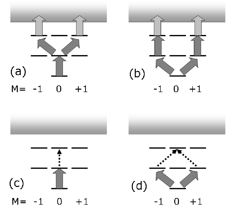
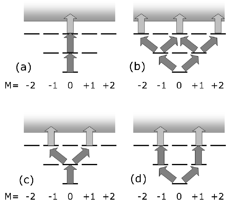
We use the polarization of the linearly polarized ionization-laser light to define the quantization axis $\hat{z}$ . Because the excitation and ionization laser beams propagate along the same axis, defined as the $x$ -axis, and light is transverse, the polarization of the excitation-laser beams can only be in the $\hat{y}$ - $\hat{z}$ plane. For a $J=1$ probed state, only $M=\pm 1$ Zeeman sublevels can be coherently excited (Fig. 3). The $M=0$ sublevel cannot be excited because the corresponding Clebsch-Gordan coefficient for a $J=1\rightarrow J^{\prime}=1$ transition is zero. For a $J=2$ probed state, three different polarizations of the state can be obtained (Fig. 4). When both excitation lasers are polarized along the $z$ -axis, the $M=0$ sublevel is populated. When one of the excitation lasers is polarized along the $z$ -axis and the other is polarized along the $y$ -axis, $M=\pm 1$ sublevels are coherently excited. When the polarizations of both lasers are along the $y$ -axis, $M=\pm 2$ and $M=0$ sublevels can be coherently excited.

III Theory

III.1 Photoionization Cross-Section

In this subsection, we show that there are at most three parameters in the total photoionization cross-section using density-matrix algebra (see, for example, Ref. Alexandrov et al. 2005; Blum 1996). Assuming that the wavelength of the ionization photons is much longer than the size of an atom, we only consider electric-dipole transitions.

The density matrix describing an ensemble of atoms in a state with total angular momentum $J$ can be expressed in the basis of its $2J+1$ Zeeman components.

	$\displaystyle\rho^{(i)}_{a}$	$\displaystyle=$	$\displaystyle\sum_{MM^{\prime}=-J}^{J}\rho_{aMM^{\prime}}^{(i)}{\left\|JM\right\rangle}{\left\langle JM^{\prime}\right\|},$		(1)
	$\displaystyle\rho_{a}$	$\displaystyle=$	$\displaystyle\frac{1}{N}\sum_{i=1}^{N}\rho^{(i)}_{a},$		(2)

where $\rho_{a~MM^{\prime}}^{(i)}$ are the coefficients in the Zeeman basis of the $i^{th}$ atom, and $\rho_{a}$ is the average density matrix of an ensemble of $N$ atoms. As we will calculate the photoionization cross-section which is normalized by the number of particles, we likewise choose the normalization

Tr[\rho_{a}]=1.

(3)

It is convenient to expand the density matrix in the basis of irreducible tensors of rank $\kappa$ ( $\kappa=0,1,\cdots,2J$ ),

\rho_{a}=\sum_{\kappa=0}^{2J}\sum_{q=-\kappa}^{\kappa}\rho^{(\kappa)}_{a~q}T^{(\kappa)}_{q},

(4)

where $T^{(\kappa)}$ are normalized polarization operators which are irreducible tensors of rank $\kappa$ with $2\kappa+1$ components $T^{(\kappa)}_{q}$ ( $q=-\kappa,-\kappa+1,\cdots,\kappa$ ), and $\rho^{(\kappa)}_{a~q}$ are coefficients, which are related to $\rho_{aMM^{\prime}}$ according to

\rho_{a~q}^{(\kappa)}=\sum_{MM^{\prime}=-J}^{J}(-1)^{J-M^{\prime}}\langle J,M,J,-M^{\prime}|\kappa,q\rangle\rho_{aMM^{\prime}},

(5)

where $\langle J,M,J,-M^{\prime}|\kappa,q\rangle$ are Clebsch-Gordan coefficients.

Photons have total angular momentum $J=1$ in the electric-dipole approximation. Therefore, the density matrix of the photons can be decomposed into irreducible tensors of ranks $\kappa=0,1$ and $2$ .

\rho_{p}=\sum_{\kappa=0}^{2}\sum_{q=-\kappa}^{\kappa}\rho^{(\kappa)}_{p~q}T^{(\kappa)}_{q},

(6)

where $\rho_{p}$ is normalized as $\rho_{a}$ .

The photoionization process is related to the density matrices of the ionizing photons and the probed state. Because total photoionization cross-section is a scalar (since we did not study the angular distribution of the ions), the irreducible tensors of the density matrix of the photons should be contracted with those of the atoms of the same ranks. The photoionization cross-section can be expressed as:

\begin{split}\sigma=&\sqrt{3(2J+1)}\left(\sigma_{0}\rho^{(0)}_{p~0}\rho^{(0)}_{a~0}+\sigma_{1}\sum_{q=-1}^{1}(-1)^{q}\rho^{(1)}_{p~q}\rho^{(1)}_{a~-q}\right.\\ &\left.+\sigma_{2}\sum_{q=-2}^{2}(-1)^{q}\rho^{(2)}_{p~q}\rho^{(2)}_{a~-q}\right),\end{split}

(7)

where $\sigma_{0,1,2}$ are coefficients determined by the atomic wavefunctions of the initial and final (continuum) states. The normalization factor $\sqrt{3(2J+1)}$ is chosen because according to Eq. (5),

	$\displaystyle\rho_{a~0}^{(0)}$	$\displaystyle=$	$\displaystyle\frac{1}{\sqrt{2J+1}},$		(8)
	$\displaystyle\rho_{p~0}^{(0)}$	$\displaystyle=$	$\displaystyle\frac{1}{\sqrt{3}}.$		(9)

Therefore, we conclude that in general there are at most three parameters in the photoionization cross-section. (There is only one parameter for a $J=0$ state and there are two parameters for a $J=1/2$ state.) For an unpolarized initial atomic state or/and an unpolarized ionization light source,¹¹ 1 Here the unpolarized light source means that the diagonal elements of the density matrix of the light are equal and the off-diagonal elements are all zero. A directional light beam cannot be unpolarized in this definition because of the lack of the polarization along its propagation direction. Such light that can be “unpolarized” in the sense of the common definition through Stokes’ parameters, in fact, possesses alignment along the propagation direction. the photoionization cross-section is $\sigma_{0}$ . If both of atoms and light are polarized, the cross-section may be different depending on their relative orientation ( $\sigma_{1}$ ) and their relative alignment ( $\sigma_{2}$ ).

III.2 Formulae for $\sigma_{0,1,2}$

In this subsection, we derive general formulae for $\sigma_{0,1,2}$ for states of arbitrary angular momenta. Consider an ensemble of atoms prepared in a particular Zeeman sublevel of the probed state ${\left|aJM\right\rangle}$ , where $a$ represents all other quantum numbers of the state, which are ionized by left-circularly polarized photons. The density matrix of the photons is

\begin{array}[]{c}\begin{array}[]{ccccc}&&M=+1&~M=0&M=-1\end{array}\\ \begin{array}[]{c}M=+1\\ M=0\\ M=-1\end{array}\left(\begin{array}[]{ccc}~~~~~1&~~~~~0&~~~~~0\\ 0&0&0\\ 0&0&0\\ \end{array}\right).\end{array}

(10)

Using Eq. (5), we can decompose it into irreducible tensors with components $\rho_{p~q}^{(\kappa)}$ :

\begin{array}[]{cc}\kappa&(q=-\kappa,\cdots,\kappa)\\ 0&\left(\frac{1}{\sqrt{3}}\right)\\ 1&\left(0,\frac{1}{\sqrt{2}},0\right)\\ 2&\left(0,0,\frac{1}{\sqrt{6}},0,0\right).\end{array}

(11)

All elements of the density matrix of the probed state are zero except $\rho_{aMM}=1$ . Using Eq. (5), we can decompose it into irreducible tensors with components $\rho_{a~q}^{(\kappa)}$ :

\begin{array}[]{cc}\kappa&(q=-\kappa,\cdots,\kappa)\\ 0&\left((-1)^{J-M}\begin{pmatrix}J&J&0\\ M&-M&0\end{pmatrix}\right)\\ 1&\left(0,(-1)^{J-M}\sqrt{3}\begin{pmatrix}J&J&1\\ M&-M&0\end{pmatrix},0\right)\\ 2&\left(0,0,(-1)^{J-M}\sqrt{5}\begin{pmatrix}J&J&2\\ M&-M&0\end{pmatrix},0,0\right).\end{array}

(12)

According to Eq. (7) the photoionization cross-section is

\begin{split}\sigma=&\sqrt{3(2J+1)}\left(\sigma_{0}\frac{(-1)^{J-M}}{\sqrt{3}}\begin{pmatrix}J&J&0\\ M&-M&0\end{pmatrix}\right.\\ &+\sigma_{1}(-1)^{J-M}\sqrt{\frac{3}{2}}\begin{pmatrix}J&J&1\\ M&-M&0\end{pmatrix}\\ &\left.+\sigma_{2}(-1)^{J-M}\sqrt{\frac{5}{6}}\begin{pmatrix}J&J&2\\ M&-M&0\end{pmatrix}\right).\end{split}

(13)

It is convenient to introduce a function $Z$ defined as:

Z(l)=\sum_{M=-J}^{J}(-1)^{J+M}\begin{pmatrix}J&J&l\\ M&-M&0\end{pmatrix}\sigma.

(14)

Using the identity of

\sum_{M=-J}^{J}\begin{pmatrix}J&J&\kappa\\ M&-M&0\end{pmatrix}\begin{pmatrix}J&J&l\\ M&-M&0\end{pmatrix}=\frac{1}{2l+1}\delta_{\kappa l},

(15)

it can be shown that

$\displaystyle Z(l=0)$	$\displaystyle=$	$\displaystyle\sqrt{2J+1}\sigma_{0},$
$\displaystyle Z(l=1)$	$\displaystyle=$	$\displaystyle\sqrt{\frac{2J+1}{2}}\sigma_{1},$	(16)
$\displaystyle Z(l=2)$	$\displaystyle=$	$\displaystyle\sqrt{\frac{2J+1}{10}}\sigma_{2}.$

From Ref. Sobel’man 1992, the photoionization cross-section can be expressed as

\sigma=\frac{4\pi^{2}m_{e}}{\hbar^{2}}\frac{k}{p}\sum_{n}|\left\langle\psi_{n}\left|\bf D^{1}_{q}\right|\psi_{a}\right\rangle|^{2},

(17)

where $m_{e}$ is the mass of the electron, $k$ is the momentum of an ionizing photon, $p$ is the momentum of an ionized electron, $\psi_{a}$ is the atomic wavefunction of the probed state and $\psi_{n}$ is the wavefunction of the coupled continuum state.

Using the relation

	$\displaystyle\|\left\langle nJ_{n}M+1\left\|\rm\bf D^{(1)}_{1}\right\|aJM\right\rangle\|^{2}$	(18)
$\displaystyle=$	$\displaystyle-\begin{pmatrix}J_{n}&1&J\\ -M-1&1&M\end{pmatrix}\begin{pmatrix}J&1&J_{n}\\ -M&-1&M+1\end{pmatrix}$
	$\displaystyle\cdot\|\left(nJ_{n}\\|{\rm\bf D}\\|aJ\right)\|^{2},$

the photoionization cross-section in the example we are considering can be written as

\sigma=-\sum_{n}A_{n}\cdot\begin{pmatrix}J_{n}&1&J\\ -M-1&1&M\end{pmatrix}\begin{pmatrix}J&1&J_{n}\\ -M&-1&M+1\end{pmatrix},

(19)

where $A_{n}=\frac{4\pi^{2}m_{e}k}{\hbar^{2}p}\cdot|\left(nJ_{n}\|{\rm\bf D}\|aJ\right)|^{2}$ . Using Eq. (19) to calculate $Z$ defined in Eq. (14),

$\displaystyle Z(l)$	$\displaystyle=$	$\displaystyle\sum_{n}A_{n}\cdot\sum_{M}(-1)^{J+M+1}\begin{pmatrix}J_{n}&1&J\\ -M-1&1&M\end{pmatrix}$	(20)
		$\displaystyle\cdot\begin{pmatrix}J&1&J_{n}\\ -M&-1&M+1\end{pmatrix}\begin{pmatrix}J&J&1\\ M&-M&0\end{pmatrix}$
	$\displaystyle=$	$\displaystyle\sum_{n}A_{n}\cdot(-1)^{J-J_{n}}\begin{pmatrix}1&1&1\\ 1&-1&0\end{pmatrix}\begin{Bmatrix}1&1&l\\ J&J&J_{n}\end{Bmatrix},~~~$

where, in the last line, we have used the identity

	$\displaystyle\sum_{m_{4}m_{5}m_{6}}(-1)^{j_{4}+j_{5}+j_{6}-m_{4}-m_{5}-m_{6}}\begin{pmatrix}j_{1}&j_{5}&j_{6}\\ m_{1}&-m_{5}&m_{6}\end{pmatrix}$	(21)
	$\displaystyle\cdot\begin{pmatrix}j_{4}&j_{2}&j_{6}\\ m_{4}&m_{2}&-m_{6}\end{pmatrix}\begin{pmatrix}j_{4}&j_{5}&j_{3}\\ -m_{4}&m_{5}&m_{3}\end{pmatrix}$
$\displaystyle=$	$\displaystyle\begin{pmatrix}j_{1}&j_{2}&j_{3}\\ m_{1}&m_{2}&m_{3}\end{pmatrix}\begin{Bmatrix}j_{1}&j_{2}&j_{3}\\ j_{4}&j_{5}&j_{6}\end{Bmatrix}.$

Comparing Eq. (20) with Eq. (16), we can derive the formulae for $\sigma_{0,1,2}$ ,

$\displaystyle\sigma_{0}$	$\displaystyle=$	$\displaystyle\sum_{n}A_{n}\cdot\frac{(-1)^{1-2J_{n}}}{3(2J+1)},$	(22)
$\displaystyle\sigma_{1}$	$\displaystyle=$	$\displaystyle\sum_{n}A_{n}\cdot\frac{(-1)^{J-J_{n}}}{\sqrt{3(2J+1})}\begin{Bmatrix}1&1&1\\ J&J&J_{n}\end{Bmatrix},$	(23)
$\displaystyle\sigma_{2}$	$\displaystyle=$	$\displaystyle\sum_{n}A_{n}\cdot\frac{(-1)^{J+J_{n}}}{\sqrt{3(2J+1})}\begin{Bmatrix}1&1&2\\ J&J&J_{n}\end{Bmatrix}.$	(24)

If the probed state is dominantly coupled to continuum states with a specific total angular momentum $J_{n}=J_{c}$ , the ratios between photoionization cross-sections are

	$\displaystyle\frac{\sigma_{1}}{\sigma_{0}}$	$\displaystyle=$	$\displaystyle(-1)^{J+J_{c}-1}\sqrt{3(2J+1)}\begin{Bmatrix}1&1&1\\ J&J&J_{c}\end{Bmatrix},$		(25)
	$\displaystyle\frac{\sigma_{2}}{\sigma_{0}}$	$\displaystyle=$	$\displaystyle(-1)^{J-J_{c}-1}\sqrt{3(2J+1)}\begin{Bmatrix}1&1&2\\ J&J&J_{c}\end{Bmatrix}.$		(26)

In Table 1, we list the ratios between $\sigma_{0,1,2}$ of a probed state with total angular momentum $J=1,2$ if it is dominantly coupled to continuum states with total angular momentum $J_{c}$ .

$J$	$J_{c}$	$\sigma_{0}$	:	$\sigma_{1}$	:	$\sigma_{2}$
	0	1	:	-1	:	1
1	1	1	:	- $\frac{1}{2}$	:	- $\frac{1}{2}$
	2	1	:	$\frac{1}{2}$	:	$\frac{1}{10}$
	1	1	:	- $\sqrt{\frac{3}{4}}$	:	$\sqrt{\frac{7}{20}}$
2	2	1	:	- $\sqrt{\frac{1}{12}}$	:	- $\sqrt{\frac{7}{20}}$
	3	1	:	$\sqrt{\frac{1}{3}}$	:	$\sqrt{\frac{1}{35}}$

Table 1: Ratios between photoionization cross-sections. The ratios are calculated assuming that a probed state with total angular momentum

J

is dominantly coupled to continuum states with total angular momentum

J_{c}

III.3 Ion-Signal Model

In this subsection, we derive a formula describing the relation between the ion signal and the photon fluence (the total photon number per unit area) of the ionization-laser pulse, taking into account the finite radiative lifetime of the probed state.

The change of the number of atoms ( $N$ ) in the probed state is due to the photoionization process and the spontaneous decay:

dN=-s(t)\sigma Ndt-\frac{N}{\tau}dt,

(27)

where $s(t)$ is the temporal distribution of the photon number intensity of the ionization-laser pulse, $\sigma$ is the photoionization cross-section, and $\tau$ is the radiative lifetime of the probed state. Assume that the ionization-laser pulse comes into the interaction region at $t=0$ and $N(t=0)=N_{0}$ . Integrating Eq. (27), for $t>0$ , we get

N(t)=N_{0}e^{-\sigma\int_{0}^{t}s(t^{\prime})dt^{\prime}}e^{-t/\tau}.

(28)

The number of ions detected after the pulse ( $N_{\rm ion}(t\rightarrow\infty)$ ) is

N_{\rm ion}=\int_{0}^{\infty}s(t)\sigma N(t)dt.

(29)

We model the temporal distribution of the photon number intensity of the ionization-laser pulse with a square function, i.e.

s(t)=\left\{\begin{array}[]{ll}\frac{n}{\tau_{l}}&{\rm for~}0<t<\tau_{l},\\ 0&{\rm otherwise},\end{array}\right.

(30)

where $n$ is the photon fluence of the whole pulse and $\tau_{l}$ is the duration of the pulse. We can then derive a formula relating $N_{\rm ion}$ to $n$ :

	$\displaystyle N_{\rm ion}$	$\displaystyle=$	$\displaystyle N_{0}\frac{n\sigma}{\tau_{l}}\int_{0}^{\tau_{l}}e^{-(\sigma n/\tau_{l}+1/\tau)t}dt$		(31)
		$\displaystyle=$	$\displaystyle N_{0}\frac{\sigma n}{\sigma n+\tau_{l}/\tau}(1-e^{-\sigma n-\tau_{l}/\tau}).$		(31)

The error due to the assumption of Eq. (30) is estimated to be $\sim 4\%$ (see Section V).

IV Results and Analysis

According to Eq. (31), we determine the photoionization cross-section, $\sigma$ , by fitting the ion-signal amplitude, $V$ , as a function of the ionization-photon fluence, $n$ , with

V(n)=a~\frac{\sigma n}{\sigma n+\tau_{l}/\tau}(1-e^{-\sigma n-\tau_{l}/\tau})+b,

(32)

where we set $\tau_{l}=7$ ns, $\tau=28$ ns for $5d6d~^{3}D_{1}$ and $33$ ns for $6s7d~^{3}D_{2}$ (see APPENDIX A), $a$ is the maximum of the amplitude of the ion signal and $b$ is a background constant (Fig. 5). The background is from photoionization by the excitation lasers. The fluctuation of the ion signal is due to the variation of pulse energies of the excitation lasers leading to fluctuations in ionization probabilities by these lasers. The number of ions detected at highest ionization light powers is $\sim 2\times 10^{6}$ . This is consistent with our estimate: the number of atoms in the interaction region is $\sim 10^{9}$ atoms $\cdot$ cm ${}^{-3}\times(\pi\times 0.05^{2}$ cm ${}^{2}\times 1$ cm $)\sim 10^{7}$ atoms, at most one-third of them (in the case of total saturation for both excitation transitions) are excited to the probed state, and some of them spontaneously decay before the ionization-laser pulse arrives.²² 2 The lifetimes of the probed states are $\sim 30$ ns (see APPENDIX A) and the ionization-laser pulse arrives the interaction region $30$ ns later than the excitation laser pulses. We observe that the fluorescence signal resulting from the spontaneous decay of the probed state drops significantly when the ionization-laser pulse arrives in the interaction region. The polarization of the probed state is determined by the polarizations of the excitation lasers. The measured photoionization cross-sections with different combinations of the polarizations of the excitation lasers are listed in Table 2.

	Polarizations of the excitation lasers
state	$\hat{z}~\hat{z}$	$\hat{y}~\hat{z}$	$\hat{z}~\hat{y}$	$\hat{y}~\hat{y}$
$5d6d~^{3}D_{1}$	—	$\sigma_{0}-\sigma_{2}$		—
	—	$2.2(2)$	$1.9(2)$	—
$6s7d~^{3}D_{2}$	$\sigma_{0}+2\sqrt{\frac{5}{7}}\sigma_{2}$	$\sigma_{0}+\sqrt{\frac{5}{7}}\sigma_{2}$		$\sigma_{0}-\sqrt{\frac{5}{7}}\sigma_{2}$
	$2.0(2)$	$1.5(2)$	$1.7(2)$	$1.1(3)$

Table 2: Measured photoionization cross-sections in units of

10^{-17}

cm². The errors in the parentheses are the statistical uncertainties. For the

5d6d~^{3}D_{1}

state, in the cases of both lasers polarized in the same direction, the fluorescence signal due to spontaneous decay of the

5d6d~^{3}D_{1}

state drops significantly and no ion signal is detected.

We use the polarization direction of the linearly polarized ionization laser to define the quantization axis ( $\hat{z}$ ). The normalized density matrix for the ionization-laser light in the basis of projections of the angular momentum on the quantization axis is

\left(\begin{array}[]{ccc}0&0&0\\ 0&1&0\\ 0&0&0\end{array}\right).

(33)

Using Eq. (5), we can decompose it into irreducible tensors with components $\rho_{p~q}^{(\kappa)}$ :

\begin{array}[]{cc}\kappa&(q=-\kappa,\cdots,\kappa)\\ 0&\left(\frac{1}{\sqrt{3}}\right)\\ 1&\left(0,0,0\right)\\ 2&\left(0,0,-\sqrt{\frac{2}{3}},0,0\right).\end{array}

(34)

IV.1 The $5d6d~^{3}D_{1}$ state

Only the $M=\pm 1$ sublevels can be populated in our experimental setup. If one excitation laser is polarized along the $y$ -axis and the other is polarized along the $z$ -axis, the normalized density matrix in the Zeeman basis is

\left(\begin{array}[]{ccc}\frac{1}{2}&0&-\frac{1}{2}\\ 0&0&0\\ -\frac{1}{2}&0&\frac{1}{2}\end{array}\right).

(35)

With Eq. (5), the components of the irreducible tensors, $\rho_{a~q}^{(\kappa)}$ are

\begin{array}[]{cc}\kappa&(q=-\kappa,\cdots,\kappa)\\ 0&\left(\frac{1}{\sqrt{3}}\right)\\ 1&\left(0,0,0\right)\\ 2&\left(-\frac{1}{2},0,\frac{1}{\sqrt{6}},0,-\frac{1}{2}\right).\end{array}

(36)

From Eq. (7), the photoionization cross-section in this relative polarization is

\sigma=\sigma_{0}-\sigma_{2}.

(37)

As mentioned in the end of Section II, constrained by our experimental setup, this is the only combination of photoionization cross-sections that we can determine. As listed in Table 2, we obtained statistically consistent photoionization cross-sections with different polarizations of the excitation lasers. The average cross-section is $2.0(2)\times 10^{-17}$ cm².

If we adjust the polarizations of both excitation-laser beams to be parallel, the fluorescence signal due to the spontaneous decay of the $5d6d~^{3}D_{1}$ state to the $6s6p~^{3}P_{1}$ state detected by the PMT drops significantly (by more than a factor of $20$ ) compared to the case of parallel polarizations and almost no ion signal is detected. As the excitation transition is nearly saturated when the polarization of two excitation-laser beams are perpendicular, the residual signal may be attributed to the imperfection of the polarizer films (polarization directions and stray ellipticity are controlled within $5^{\circ}$ .)

IV.2 The $6s7d~^{3}D_{2}$ state

Three different alignments of this state were excited with different combinations of the polarizations of the two excitation lasers. Following the same approach as we used for the $5d6d~^{3}D_{1}$ state, we get that

$\displaystyle\sigma(\hat{z}\hat{z})$	$\displaystyle=$	$\displaystyle\sigma_{0}+2\sqrt{\frac{5}{7}}\sigma_{2},$	(38)
$\displaystyle\sigma(\hat{z}\hat{y})$	$\displaystyle=$	$\displaystyle\sigma(\hat{y}\hat{z})=\sigma_{0}+\sqrt{\frac{5}{7}}\sigma_{2},$	(39)
$\displaystyle\sigma(\hat{y}\hat{y})$	$\displaystyle=$	$\displaystyle\sigma_{0}-\sqrt{\frac{5}{7}}\sigma_{2}.$	(40)

Indeed, we obtained different photoionization cross-sections with different polarizations of the excitation lasers: when both excitation-laser beams are polarized along the $\hat{z}$ -axis, $\sigma=2.0(2)$ ; when both are polarized along the $\hat{y}$ -axis, $\sigma=1.1(3)$ ; when one along $\hat{y}$ and one along $\hat{z}$ , $\sigma=1.6(2)$ (Table 2). The fit shows that $\sigma_{0}=1.3(1)\times 10^{-17}$ cm² and $\sigma_{2}=0.43(8)\times 10^{-17}$ cm². The ratio $\sigma_{2}/\sigma_{0}\sim 0.34(7)$ suggests that this state is coupled most to continuum states with $J=1$ or/and $3$ (Table 1). We are not able to derive $\sigma_{1}$ because all components of the rank-one irreducible tensor for linearly polarized ionization photons are zero. If the ionization and excitation laser beams are circularly polarized, $\sigma_{1}$ can be derived. However, this was not attempted in the present work.

V Sources of Systematic error

The dominant source of the systematic error comes from our oversimplified model of the spatial profile and the temporal distribution of the intensity of the ionization-laser pulses. The spatial profile of the ionization laser is approximately Gaussian, with a diameter of $\sim 4$ mm. We measure the energy of the laser pulse that passes through the $1.01$ -mm-diameter iris and approximate the intensity as a constant. A calculation shows that this approximation may cause an maximum $(+10\%)$ correction on the photoionization cross-section. This correction is hard to estimate more accurately because the excitation and ionization transitions are partially saturated. The temporal distribution of the intensity, which is modelled as a square function, can be actually very complicated. In our case of $\tau_{l}/\tau\sim 1/4$ ( $\tau_{l}\sim 7$ ns and $\tau\sim 30$ ns), a numerical calculation shows that the variation of the fit cross-section is within $4\%$ with several trial functions for the temporal distribution.

A secondary source of the systematic error comes from the measurement of the ionization-photon fluence, including the $5\%$ uncertainty on the calibration function of the photodiode used as an energy meter and the $4\%$ uncertainty on the opening size of the iris.

The barium sample used has natural isotopic abundance. The barium isotopes with non-zero nuclear spin (¹³⁵Ba, $6.59\%$ , and ¹³⁷Ba, $11.23\%$ , both with nuclear spin $I=3/2$ ) have hyperfine structure Jitschin and Meisel 1980. We have modelled a possible effect due to hyperfine quantum beats (see, for example, Haroche 1976) in both the $6s6p~^{1}P_{1}$ intermediate state, and the states we photoionize. We find that this effect from $\sim 18\%$ of our Ba sample can cause a maximum $6\%$ correction on the photoionization cross-section. The correction is hard to estimate more accurately because of the lack of the knowledge of the temporal distribution of the ionization laser intensity. Other sources of systematic error, including the determination of the polarizations of the laser beams ( $<2\%$ ) and the nonlinearity of the photodiode ( $<2\%$ ), are found to be negligible. Overall, all the photoionization cross-sections measured in this work have a systematic uncertainty of $\sim 13\%$ . In Table 3, we have listed all experimental results measured in this work with systematic and statistical errors.

state	photoionization cross-sections
$5d6d~^{3}D_{1}$	$\sigma_{0}-\sigma_{2}=2.0(3)\times 10^{-17}$ cm²
$6s7d~^{3}D_{2}$	$\sigma_{0}=1.3(2)\times 10^{-17}$ cm²
	$\sigma_{2}=0.43(9)\times 10^{-17}$ cm²
	$\sigma_{2}/\sigma_{0}=0.34(7)$

Table 3: Measured photoionization cross-sections with systematic and statistical errors combined.

VI Conclusion

In this work, we have measured the photoionization cross-sections of the $5d6d~^{3}D_{1}$ and $6s7d~^{3}D_{2}$ states of Ba with the ionization-laser wavelength $556.6$ nm. We found that the photoionization cross-section of the $6s7d~^{3}D_{2}$ state depends on the relative polarizations of the atomic state and the ionization-laser beam. We have introduced a general tensor formalism of polarization-dependent photoionization cross-sections and determined two of the three parameters of the photoionization cross-section of the $6s7d~^{3}D_{2}$ state.

Acknowledgements.

The authors wish to thank D. English and S. M. Rochester for help with the experiments and useful discussions, and D. Angom, M. Auzinsh, R. deCarvalho, M. Havey, J. Higbie, D. Kleppner, M. G. Kozlov and J. E. Stalnaker for helpful advice. This research was supported by the National Science Foundation.

Appendix A Radiative lifetime measurement

In section IV, it has been shown that the temporal evolution of ion signals studied in this work depends on the radiative lifetimes of the probed states. Using almost the same experimental setup, we have measured the radiative lifetimes of five even-parity excited states of Ba.

The barium atoms in an atomic beam, with estimated density of $\sim 10^{9}$ atoms $/$ cm³ in the interaction region, are excited by pulsed lasers to the even-parity states of interest via two E1 transitions. For different probed states, different combinations of the lasers, including a frequency-doubled Nd:YAG laser (wavelength $\sim 532$ nm) and dye lasers with Rhodamine 6G (wavelength $556-570$ nm) or Fluorescein 548 (wavelength $546-567$ nm), are used for the excitation. Some states of interest may be probed by different combinations of lasers as a check of consistency. In some cases of lifetime measurement, atoms can be first excited to the $6s6p~^{1}P_{1}$ state efficiently by the amplified spontaneous emission (ASE) of the dye laser because the transition probability of $6s^{2}~{}^{1}S_{0}\rightarrow 6s6p~^{1}P_{1}$ is large; therefore, only one dye laser is used to excite a two-step E1-E1 transition.

Fluorescence resulting from spontaneous decay to a lower-lying odd-parity state was detected with a PMT. A colored-glass filter was used to reduce scattered light from the lasers, interference filters with $10$ -nm bandwidth were used to select the decay channel of interest and a linear-polarizing film was used to select a polarization of the fluorescence. We recorded the time-dependent fluorescence signals with a digital oscilloscope and analyzed data with a personal computer running the Mathematica program. We recorded fluorescence signals without averaging because we found that the averaging in general elongates the apparent lifetime and the fitted lifetime is sensitive to the number of the averaged samples. This is probably the result of jitter in the triggering of the oscilloscope and/or the lasers.

We determine the radiative lifetime of a probed state by fitting the fluorescence signal due to spontaneous decay with an exponential function:

f(t)=a~e^{-t/\tau}+b,{\rm~for~}t\geq 0,

(41)

where $a$ is the signal amplitude, $\tau$ is the radiative lifetime of the probed state, $b$ is the constant background and the probed state is populated at $t=0$ (Fig. 6). It can be shown (APPENDIX B) that we can avoid the effects of the finite PMT response time, the finite laser pulse width and the finite oscilloscope response time if only the data points with time sufficiently long after the laser excitation are used in the fitting.

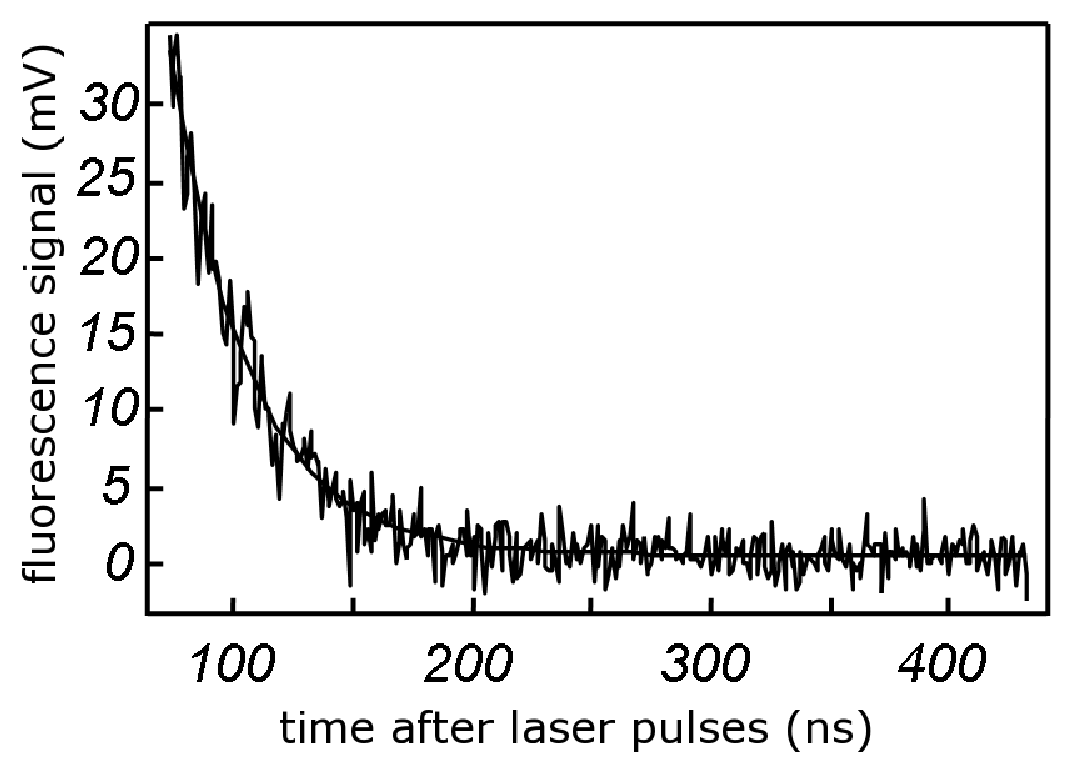
In the data analysis, only data points later than a certain time, $t_{0}(>0)$ , were fit to an exponential function. The fitted lifetime may vary with $t_{0}$ if $t_{0}$ is not sufficiently long. As $t_{0}$ increases, the fitted lifetime will approach a consistent value, which means that the effects of PMT response etc. become negligible (Fig. 7). If $t_{0}$ is chosen too long, there is no signal left to fit. Typically, we found that when $t_{0}$ is greater than $\sim 75$ ns, the fitting gives a consistent lifetime.

The lifetimes determined in this work are listed in Table 4. The lifetimes of the same probed states were measured from the fluorescence signals with different excitation schemes (different combinations of lasers or ASE) and different detection schemes (different IFs and/or different orientation of the polarizing film). The fitting gives consistent results. Comparing this work with previous experiments, we found that the lifetimes of the $6s7d~^{3}D_{2}$ and $6s7d~^{3}D_{1}$ states disagree with those reported in Ref. Smedley and Marran 1993 by more than two standard deviations. The lifetimes of $5d6d~^{3}S_{1}$ and $5d6d~^{3}D_{1}$ states agree with the previous results within one standard deviation Smedley and Marran 1993; Derr 1997.

		Lifetime (ns)
Upper state	Lower state	this work	previous work
$6s7d~^{3}D_{2}$	$6s6p~^{3}P_{1}$	33(2)	39.0(18) Smedley and Marran 1993
$6s7d~^{3}D_{1}$	$6s6p~^{3}P_{1}$	34(2)	39.0(12) Smedley and Marran 1993
$5d6d~^{3}S_{1}$	$6s6p~^{3}P_{2}$	25(2)	25(15) Derr 1997
$5d6d~^{3}D_{1}$	$6s6p~^{3}P_{1}$	28(5)	23.0(18) Smedley and Marran 1993
$5d6d~^{3}D_{2}$	$6s6p~^{3}P_{2}$	23(2)

Table 4: Radiative lifetimes determined in this work. The presented errors of lifetimes determined in this work include statistical and systematic uncertainties.

Hyperfine quantum beats are a potential source of systematic error for lifetime measurements. Our simulation shows that there can be a maximum $3\%$ systematic error on the radiative lifetime if we fit the fluorescence signal with an exponential function. Other sources of systematic errors may result from the finite response time, afterpulses and nonlinearity of the PMT. We found that these systematic uncertainties can be minimized $<1\%$ , which is much smaller than statistical uncertainties, by appropriate experimental procedure. To avoid any possible detection of unexpected cascade fluorescence channels with wavelength “coincidentally” close to the target fluorescence, we have searched all the possible decay transitions according to the latest updated energy levels of neutral barium Curry 2004.³³ 3 All the energy levels of barium below the probe states have been identified except the $5d^{2}~{}^{1}G_{4}$ state. Transitions to this state from the levels of interest are forbidden by the angular-momentum selection rules. No cascade decay channels of the probed state were found to be detectable. We have also used different IFs for the same decay channels. They all give a consistent lifetime. In the data analysis, we also subtract the temporal fluorescence data by off-resonance data to eliminate the effect of the scattered light and any off-resonance interactions.

Appendix B PMT and Oscilloscope Response

The PMT used in this work has a rise time of $\sim 8$ ns and a response time of $\sim 15$ ns FWHM. The oscilloscope bandwidth is $500$ MHz. The temporal width of the laser pulse is about $7$ ns. The lifetimes of the probed states are all less than $40$ ns. Therefore, the systematic effect due to these finite responses should be considered. We prove that this effect becomes negligible if only data points with time sufficiently long after the laser pulses are considered.

The fluorescence signal due to a spontaneous decay can be expressed as an exponential function:

F(t)=\left\{\begin{array}[]{ll}0,&{\rm~for~}t<0\\ e^{-t/\tau},&{\rm~for~}t\geq 0\end{array},\right.

(42)

where $\tau$ is the radiative lifetime of the probed state and the probed state is prepared at $t=0$ .

Assume that after a sharp light pulse, the PMT signal follows an exponential decay function. We can model the PMT response with the following function:

R(t)=\left\{\begin{array}[]{ll}0,&{\rm~for~}t<0\\ P(t)\ e^{-t/\tau_{p}},&{\rm~for~}t>0\end{array},\right.

(43)

where $P$ is any polynomial and $\tau_{p}$ is the characteristic time of the PMT response. In this work, we have the PMT response that decays faster than the fluorescence, i.e., $\tau_{p}<\tau$ .

The signal observed on the oscilloscope, $S(t)$ , is the convolution of fluorescence signal with the PMT response function:

$\displaystyle S(t)$	$\displaystyle=$	$\displaystyle\int_{0}^{t}F(t^{\prime})R(t-t^{\prime})dt^{\prime}$	(44)
	$\displaystyle=$	$\displaystyle\int_{0}^{t}e^{-t^{\prime}/\tau}~R(t-t^{\prime})dt^{\prime}$
	$\displaystyle=$	$\displaystyle\int_{-\infty}^{t}e^{-t^{\prime}/\tau}~R(t-t^{\prime})dt^{\prime}$
		$\displaystyle-\int_{-\infty}^{0}e^{-t^{\prime}/\tau}~R(t-t^{\prime})dt^{\prime}$
	$\displaystyle\equiv$	$\displaystyle S_{1}(t)-S_{2}(t).$

To simplify $S_{1}(t)$ , we change the integrated variable $t^{\prime}$ to $t-x$ :

	$\displaystyle S_{1}(t)$	$\displaystyle=$	$\displaystyle\int_{0}^{\infty}e^{(x-t)/\tau}~R(x)dx$		(45)
		$\displaystyle=$	$\displaystyle e^{-t/\tau}\int_{0}^{\infty}e^{x(1/\tau-1/\tau_{p})}P(x)dx.$		(45)

Because $\tau_{p}$ is smaller than $\tau$ , the integral in Eq.(45) converges and is a finite constant. Therefore,

S_{1}(t)=C~e^{-t/\tau}.

(46)

The function $S_{2}(t)$ can also be simplified,

	$\displaystyle S_{2}(t)$	$\displaystyle=$	$\displaystyle\int_{-\infty}^{0}e^{-t^{\prime}/\tau}~P(t-t^{\prime})~e^{-(t-t^{\prime})/\tau_{p}}dt^{\prime}$		(47)
		$\displaystyle=$	$\displaystyle e^{-t/\tau_{p}}\int_{-\infty}^{0}e^{-t^{\prime}(1/\tau-1/\tau_{p})}~P(t-t^{\prime})dt^{\prime}.$		(47)

Because $\tau_{p}$ is smaller than $\tau$ , the integral in Eq.(47) converges and is another polynomial. Hence, we get

S_{2}(t)=P^{\prime}(t)~e^{-t/\tau_{p}}.

(48)

Using Eq. (46) and Eq. (48), we can simplify the observed signal function as

S(t)=C~e^{-t/\tau}-P^{\prime}(t)~e^{-t/\tau_{p}}.

(49)

As $t$ becomes large, the second term in Eq. (49) approaches zero faster than the first term; therefore, the effect of the PMT response becomes negligible.

References

Kelly (1990) H. P. Kelly, in AIP Conference Proceedings (1990), vol. 215 of AIP Conf. Procs., p. 292.
Lubell and Raith (1969) M. S. Lubell and W. Raith, Phys. Rev. Lett. 23, 211 (1969).
Fox et al. (1971) R. A. Fox, R. M. Kogan, and E. J. Robinson, Phys. Rev. Lett. 26, 1416 (1971).
Kogan et al. (1971) R. M. Kogan, R. A. Fox, G. T. Burnham, and E. J. Robinson, Bull. Amer. Phys. Soc. 16, 1411 (1971).
DeMille et al. (1999) D. DeMille, D. Budker, N. Derr, and E. Deveney, Phys. Rev. Lett. 83, 3978 (1999).
English et al. (2000) D. English, D. Budker, and D. DeMille, in proceedings of the International Conference on Spin-Statistics Connection and Commutation Relations: Experimental Tests and Theoretical Implications, edited by R. C. Hilborn and G. M. Tino (Anacapri, Italy, 2000), vol. 545 of AIP Conf. Procs., p. 281.
Rochester et al. (1999) S. M. Rochester, C. J. Bowers, D. Budker, D. DeMille, and M. Zolotorev, Phys. Rev. A. 59, 3480 (1999).
Li et al. (2004) C.-H. Li, S. M. Rochester, M. G. Kozlov, and D. Budker, Phys. Rev. A. 69, 042507 (2004).
Alexandrov et al. (2005) E. B. Alexandrov, M. Auzinsh, D. Budker, D. F. Kimball, S. M. Rochester, and V. V. Yashchuk, JOSA B 22(1), 7 (2005).
Blum (1996) K. Blum, Density Matrix Theory and Applications (Plenum Publishing Corporation, 233 Spring Street, New York, NY 10013, 1996).
Sobel’man (1992) I. I. Sobel’man, Atomic spectra and radiative transitions (Springer-Verlag, Berlin, 1992).
Jitschin and Meisel (1980) W. Jitschin and G. Meisel, Zeitschrift fur Physik A 295, 37 (1980).
Haroche (1976) S. Haroche, in High-resolution Laser Spectroscopy, edited by K. Shimoda (Springer-Verlag, Berlin., 1976), p. 256.
Smedley and Marran (1993) J. E. Smedley and D. F. Marran, Phys. Rev. A 47, 126 (1993).
Derr (1997) N. Derr, Undergraduate thesis, UC Berkeley. (1997).
Curry (2004) J. J. Curry, J. Phys. Chem. Ref. Data 33, 725 (2004).